Class 21: Network Sparsification, Filtering, & Thresholding

Goal of today’s class:

1. Introduce network reduction/filtering/thresholding

2. Introduce biases emerging in thresholding

3. Introduce weighted disparity filter

Acknowledgement: Parts of this lesson draws from material by Matteo Chinazzi and Qian Zhang.

Much of it is adapted from the 2024 final project of Daniel González Quezada, a PhD student in Network Science at Northeastern University!

---

1. Come in. Sit down. Open Teams.

2. Find your notebook in your /Class_21/ folder.

---

import networkx as nx
import pandas as pd
import numpy as np
import matplotlib.pyplot as plt
from matplotlib import rc
rc('axes', axisbelow=True)
rc('axes', fc='w')
rc('figure', fc='w')
rc('savefig', fc='w')

---

Real networks are often big, dense, noisy, and full of redundant connections. Airline networks, coauthorship graphs, correlation networks, and bipartite projections all generate graphs where a huge fraction of node pairs are linked by something. If we try to visualize or analyze these networks directly, we quickly run into both conceptual and computational limits: the hairball plots are unreadable, and algorithms that scale with \(|E|\) or worse (all-pairs shortest paths, betweenness, some community detection methods, large-scale simulations) become expensive.

In this chapter we study network sparsification: the problem of replacing a given graph by a much sparser graph on the same set of nodes that still behaves like the original for certain tasks. The sparsified graph should be small enough to work with comfortably, but still preserve the structures or statistics we care about: shortest paths, centralities, communities, flows, diffusion processes, and so on.

Intuitively, sparsification is about extracting a backbone or skeleton of a network: a reduced set of edges that carries most of the structural signal and discards as much redundancy and noise as possible.

G = nx.karate_club_graph()
nodes = list(G.nodes())
G_edges = list(G.edges())
pos = nx.spring_layout(G)

fig, ax = plt.subplots(1,5,figsize=(17,3),dpi=200)
plt.subplots_adjust(wspace=0.4)

nx.draw(G, pos, node_size=50, node_color='.1', edge_color='.5', width=2, ax=ax[0])
ax[0].set_title('Original network')

ax[1].set_title("...let's sparsify this network...")
ax[2].set_title("...to different extents...")
ax[3].set_title("...and see what they look like!")
ax[4].set_title('~~fun~~')


plt.show()

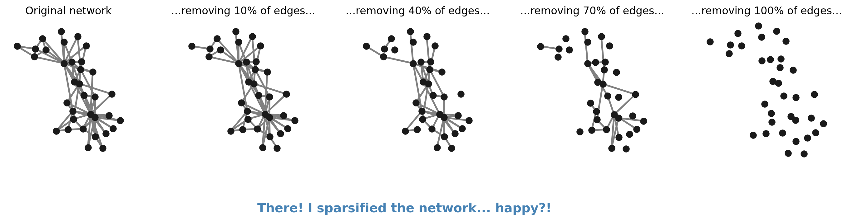
…is sparsification as easy as just… removing edges?

fig, ax = plt.subplots(1,5,figsize=(17,3),dpi=200)
plt.subplots_adjust(wspace=0.4)

nx.draw(G, pos, node_size=50, node_color='.1', edge_color='.5', width=2, ax=ax[0])
ax[0].set_title('Original network')


# remove 10% of edges
G2_edges = list(G.edges())
np.random.shuffle(G2_edges)
G2 = nx.Graph()
G2.add_nodes_from(nodes)
G2.add_edges_from(G2_edges[:int(0.9*len(G_edges))])
nx.draw(G2, pos, node_size=50, node_color='.1', edge_color='.5', width=2, ax=ax[1])
ax[1].set_title('...removing 10% of edges...')

# remove 40% of edges
G2_edges = list(G.edges())
np.random.shuffle(G2_edges)
G2 = nx.Graph()
G2.add_nodes_from(nodes)
G2.add_edges_from(G2_edges[:int(0.6*len(G_edges))])
nx.draw(G2, pos, node_size=50, node_color='.1', edge_color='.5', width=2, ax=ax[2])
ax[2].set_title('...removing 40% of edges...')

# remove 70% of edges
G2_edges = list(G.edges())
np.random.shuffle(G2_edges)
G2 = nx.Graph()
G2.add_nodes_from(nodes)
G2.add_edges_from(G2_edges[:int(0.3*len(G_edges))])
nx.draw(G2, pos, node_size=50, node_color='.1', edge_color='.5', width=2, ax=ax[3])
ax[3].set_title('...removing 70% of edges...')


# remove 100% of edges
G2_edges = list(G.edges())
np.random.shuffle(G2_edges)
G2 = nx.Graph()
G2.add_nodes_from(nodes)
G2.add_edges_from(G2_edges[:int(0.0*len(G_edges))])
nx.draw(G2, pos, node_size=50, node_color='.1', edge_color='.5', width=2, ax=ax[4])
ax[4].set_title('...removing 100% of edges...')


plt.suptitle('There! I sparsified the network... happy?!', color='steelblue', fontsize='x-large', y=-0.1, fontweight='bold')

plt.show()

Sparsification, sampling, and filtering

It is useful to distinguish sparsification from a few closely related ideas that appear in other parts of the course.

Sampling asks how to select a subset of nodes or edges when we cannot or do not want to observe the full graph. The sampled graph is mainly a tool for estimating properties of an underlying, unobserved network.

Filtering and thresholding start from a weighted graph and ask which edges are statistically meaningful. Methods like disparity filters or likelihood-based backbones treat weights as noisy measurements, compare them to a null model, and keep only edges whose weights are unexpectedly large. The goal is to identify significant ties, not necessarily to approximate every structural aspect of the original network.

Sparsification assumes we already have the full graph and want to construct a smaller graph on the same nodes that approximates the original. Here we are not trying to estimate an unknown network; instead, we are constructing a surrogate graph that is cheaper to store, visualize, and analyze, while still supporting similar results for specific downstream tasks.

A convenient way to think about sparsification is as a two-step “score + filter” procedure:

1. Assign each edge \(e \in E\) an importance score \(s(e)\) based on some structural criterion (degree of its endpoints, neighborhood overlap, effective resistance, etc.).

2. Select a reduced edge set \(E' \subset E\) using a global or local rule (for example, keep the top \(q\) fraction of edges overall, or keep only the top \(k\) edges incident to each node).

Most practical sparsification methods can be understood as choices of scoring function and filtering rule.

---

What does it mean to approximate a graph?

A sparsifier of a graph \(G = (V,E)\) is another graph \(H = (V,E')\) on the same node set (usually) \(|V(H)| = |V(G)|\) and a much smaller edge set \(|E'| \ll |E|\) that approximates \(G\) with respect to some property of interest. Different choices of property lead to different notions of sparsification. In principle, it is possible to compress a dense graph down to \(O(n \log n)\) edges while still preserving strong global properties. In practice, however, such algorithms can be too heavy for everyday data analysis, and the property we care most about is usually much more specific than “all cuts” or “all quadratic forms”. This motivates simpler, task-driven sparsifiers that are easier to implement and reason about.

edges = pd.read_csv('data/openflights_USairport_2010.txt', sep=' ', header=None,
                    names=['source','target','weight'])
nodes = pd.read_csv('data/openflights_airports.txt', sep=' ')


w_edge_dict = dict(zip(list(zip(edges['source'],edges['target'])), edges['weight']))

G = nx.Graph()
G.add_nodes_from(nodes['Airport ID'].values)
G.add_edges_from([(int(i),int(j),{'weight':k}) for i,j,k in list(edges.values)])

Gx = nx.subgraph(G, max(nx.connected_components(G), key=len))

N = G.number_of_nodes()
M = G.number_of_edges()
print("Number of Airports:", N)
print("Number of Connections:", M)

Number of Airports: 6675
Number of Connections: 17215

pos = dict(zip(nodes['Airport ID'].values, list(zip(nodes['Longitude'],nodes['Latitude']))))

for x in [i for i in G.nodes() if i not in pos.keys()]:
    try:
        pos[x] = pos[x+1]
    except:
        pos[x] = pos[x-1]

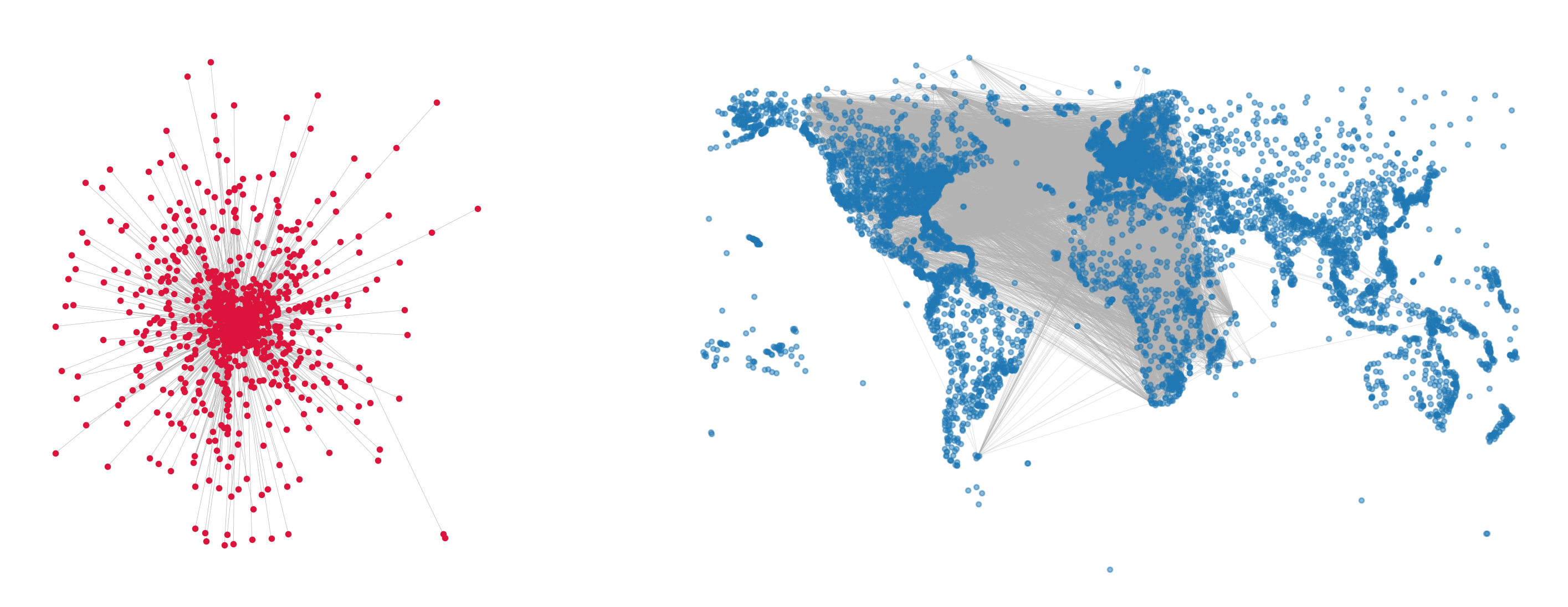
fig, ax = plt.subplots(1,2,figsize=(18,7),
                       gridspec_kw={'width_ratios':[2,3.5]},
                       dpi=200)

nx.draw(Gx, node_size=10, edge_color='.7', width=0.25, ax=ax[0], node_color='crimson')


nx.draw(G, pos={i:pos[i] for i in G.nodes()}, node_size=10,
        edge_color='.7', width=0.25, ax=ax[1], alpha=0.5)


plt.show()

def get_binning(data, num_bins=40, is_pmf=False, log_binning=False, threshold=0):
    """
    Bins the input data and calculates the probability mass function (PMF) or 
    probability density function (PDF) over the bins. Supports both linear and 
    logarithmic binning.

    Parameters
    ----------
    data : array-like
        The data to be binned, typically a list or numpy array of values.
    num_bins : int, optional
        The number of bins to use for binning the data (default is 15).
    is_pmf : bool, optional
        If True, computes the probability mass function (PMF) by normalizing 
        histogram counts to sum to 1. If False, computes the probability density 
        function (PDF) by normalizing the density of the bins (default is True).
    log_binning : bool, optional
        If True, uses logarithmic binning with log-spaced bins. If False, uses 
        linear binning (default is False).
    threshold : float, optional
        Only values greater than `threshold` will be included in the binning, 
        allowing for the removal of isolated nodes or outliers (default is 0).
    
    Returns
    -------
    x : numpy.ndarray
        The bin centers, adjusted to be the midpoint of each bin.
    p : numpy.ndarray
        The computed PMF or PDF values for each bin.
    
    Notes
    -----
    This function removes values below a specified threshold, then defines 
    bin edges based on the specified binning method (linear or logarithmic). 
    It calculates either the PMF or PDF based on `is_pmf`.
    """
    
    # Filter out isolated nodes or low values by removing data below threshold
    values = list(filter(lambda x: x > threshold, data))
#     if len(values) != len(data):
#         print("%s isolated nodes have been removed" % (len(data) - len(values)))

    # Define the range for binning (support of the distribution)
    lower_bound = min(values)
    upper_bound = max(values)

    # Define bin edges based on binning type (logarithmic or linear)
    if log_binning:
        # Use log-spaced bins by taking the log of the bounds
        lower_bound = np.log10(lower_bound)
        upper_bound = np.log10(upper_bound)
        bin_edges = np.logspace(lower_bound, upper_bound, num_bins + 1, base=10)
    else:
        # Use linearly spaced bins
        bin_edges = np.linspace(lower_bound, upper_bound, num_bins + 1)

    # Calculate histogram based on chosen binning method
    if is_pmf:
        # Calculate PMF: normalized counts of data in each bin
        y, _ = np.histogram(values, bins=bin_edges, density=False)
        p = y / y.sum()  # Normalize to get probabilities
    else:
        # Calculate PDF: normalized density of data in each bin
        p, _ = np.histogram(values, bins=bin_edges, density=True)

    # Compute bin centers (midpoints) to represent each bin
    x = bin_edges[1:] - np.diff(bin_edges) / 2  # Bin centers for plotting

    # Remove bins with zero probability to avoid plotting/display issues
    x = x[p > 0]
    p = p[p > 0]

    return x, p

# Plot degree and strength distributions
fig, ax = plt.subplots(1,2,figsize=(12,4),dpi=200)
plt.subplots_adjust(wspace=0.25)

x, y = get_binning(list(dict(G.degree()).values()),
                   num_bins=20, log_binning=True)
ax[0].loglog(x,y,'o',color='crimson')
ax[0].set_ylabel(r'$P(k)$',fontsize='x-large')
ax[0].set_xlabel(r'$k$',fontsize='x-large')
ax[0].set_title('Degree distribution')

x, y = get_binning(list(dict(G.degree(weight='weight')).values()),
                   num_bins=20, log_binning=True)
ax[1].loglog(x,y,'o',color='steelblue')
ax[1].set_ylabel(r'$P(s)$',fontsize='x-large')
ax[1].set_xlabel(r'$s$',fontsize='x-large')
ax[1].set_title('Strength distribution')

plt.suptitle('OpenFlights Data',fontweight='bold',y=1.0)

plt.show()

---

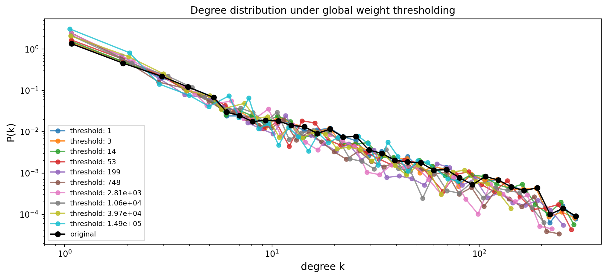
Sparsification Method: Global Thresholding

One of the most common ways to sparsify a weighted network is to apply a single global threshold on edge weights:

• keep edges with weight \(w_{ij} > \tau\),

• drop edges with weight \(w_{ij} \le \tau\).

This kind of global thresholding is easy to implement and often appears as a first preprocessing step for correlation networks, co-occurrence networks, or projected bipartite graphs.

However, it comes with serious drawbacks:

• It ignores/destroys heterogeneity in the network. Nodes with very small total strength (or low degrees) are disproportionately likely to lose all their edges when we apply a single global cutoff.

• It ignores local multi-scale structure. A single value of \(\tau\) cannot preserve both strong ties between hubs and weaker—but locally important—ties between low-strength nodes.

• It tends to distort degree and strength distributions in ways that are hard to control, especially when edge weights span several orders of magnitude and lack a characteristic scale.

In the code below we implement a simple thresholding function and then explore how gradually increasing the weight threshold reshapes the degree and edge weight distributions of a weighted graph.

Your turn!

def threshold_graph(G, threshold):
    """
    Return a globally thresholded version of a weighted graph.

    The function constructs a new graph H on (optionally) the same node set as G
    and keeps only those edges whose weight exceeds a global threshold.

    Parameters:
        G: A NetworkX graph with edge weights stored under `weight_key`.
        threshold: Global cutoff value. Only edges with weight > threshold
            are retained.

    Returns:
        G_thresh: A new NetworkX graph containing the thresholded edge set.
    """

    

    pass
    
#     return G_thresh

---

def threshold_graph(G, threshold, weight_key="weight", copy_nodes=True):
    """
    Return a globally thresholded version of a weighted graph.

    The function constructs a new graph H on (optionally) the same node set as G
    and keeps only those edges whose weight exceeds a global threshold.

    Parameters:
        G: A NetworkX graph with edge weights stored under `weight_key`.
        threshold: Global cutoff value. Only edges with weight > threshold
            are retained.
        weight_key: Name of the edge attribute used as weight (default: "weight").
        copy_nodes: If True, copy all nodes (and their attributes) from G into H
            even if they become isolated. If False, only nodes incident to
            retained edges will appear in H.

    Returns:
        H: A new NetworkX graph containing the thresholded edge set.
    """
    H = G.__class__()  # preserve directed / undirected type

    if copy_nodes:
        H.add_nodes_from(G.nodes(data=True))

    for u, v, data in G.edges(data=True):
        w = data.get(weight_key)
        if w is None:
            continue
        if w > threshold:
            # keep all existing edge attributes
            H.add_edge(u, v, **data)

    return H

edges = pd.read_csv('data/openflights_USairport_2010.txt', sep=' ', header=None,
                    names=['source','target','weight'])
nodes = pd.read_csv('data/openflights_airports.txt', sep=' ')


w_edge_dict = dict(zip(list(zip(edges['source'],edges['target'])), edges['weight']))

G = nx.Graph()
G.add_nodes_from(nodes['Airport ID'].values)
G.add_edges_from([(int(i),int(j),{'weight':k}) for i,j,k in list(edges.values)])

Gx = nx.subgraph(G, max(nx.connected_components(G), key=len))

# Collect original edge weights
weights = list(nx.get_edge_attributes(G, "weight").values())
weights = np.array(weights)

min_w = weights.min()
max_w = weights.max()

# Use logarithmically spaced thresholds between min_w and max_w / 10
w_thresholds = np.logspace(np.log10(min_w),
                           np.log10(max_w) - 1,
                           10).astype(int)

fig, ax = plt.subplots(1,1,figsize=(12,5),dpi=200)

for w_threshold in w_thresholds:
    G_filtered = threshold_graph(Gx, w_threshold)
    frac_nodes = 100.0 * G_filtered.number_of_nodes() / float(N)

#     print(f"w_threshold: {w_threshold:.6g} ({frac_nodes:5.2f}% of nodes remain)")

    degrees_filtered = list(dict(G_filtered.degree()).values())
    x, y = get_binning(degrees_filtered, log_binning=True)
    ax.loglog(x, y, "o-", label=f"threshold: {w_threshold:.3g}", ms=5, alpha=0.8)

# Original degree distribution
x_true, y_true = get_binning(list(dict(G.degree()).values()), log_binning=True)
ax.loglog(x_true, y_true, "-o", label="original", color='k')

ax.set_xlabel("degree k", fontsize='large')
ax.set_ylabel("P(k)", fontsize='large')
ax.set_title("Degree distribution under global weight thresholding")
ax.legend(fontsize='small', loc=3)

plt.show()

fig, ax = plt.subplots(1,1,figsize=(12,5),dpi=200)

for w_threshold in w_thresholds:
    G_filtered = threshold_graph(Gx, w_threshold)
    frac_nodes = 100.0 * G_filtered.number_of_nodes() / float(N)

#     print(f"w_threshold: {w_threshold:.6g} ({frac_nodes:5.2f}% of nodes remain)")

    weights_filtered = list(nx.get_edge_attributes(G_filtered, "weight").values())
    if len(weights_filtered) == 0:
        continue  # nothing left at this threshold

    x, y = get_binning(weights_filtered, log_binning=True)
    ax.loglog(x, y, "o-", label=f"threshold: {w_threshold:.3g}", ms=5, alpha=0.8)

# Original weight distribution
weights_original = list(nx.get_edge_attributes(G, "weight").values())
x_true, y_true = get_binning(weights_original, log_binning=True)
ax.loglog(x_true, y_true, "-o", label="original", color='k')

plt.xlabel("edge weight w", fontsize='large')
plt.ylabel("P(w)", fontsize='large')
plt.title("Edge weight distribution under global weight thresholding")
plt.legend(fontsize='small', loc=3)

plt.show()

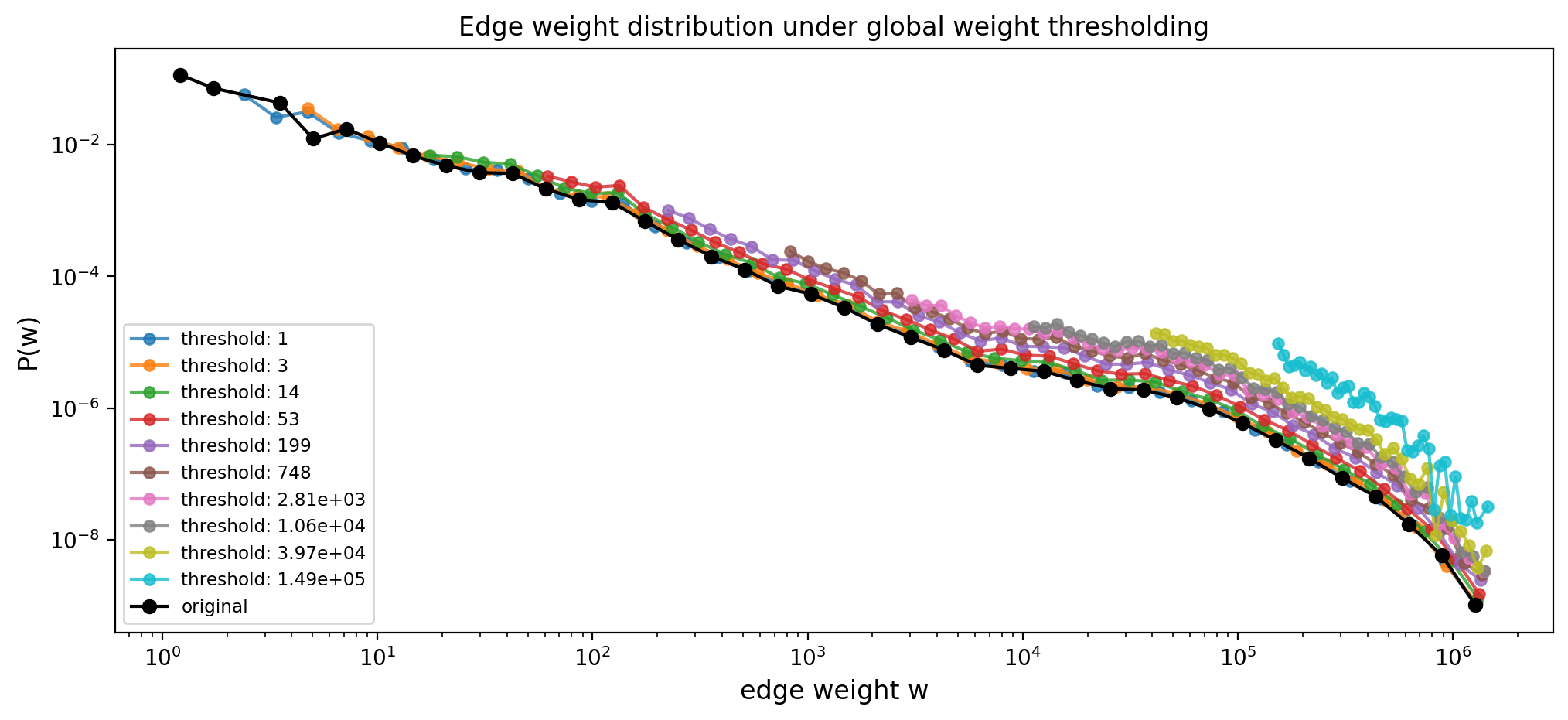
Maybe thresholding is too blunt…

Thresholding really chops off a lot of the network’s information

---

Sparsification Method: Spanning Trees

A spanning tree of a connected graph \(G = (V, E)\) is a subgraph \(T = (V, E_T)\) that:

1. contains all the nodes of \(G\) (it “spans” \(V\)), and

2. is a tree, i.e. it is connected and has no cycles.

Every spanning tree has exactly \(|V| - 1\) edges. When the graph is weighted, we can look for spanning trees that are optimal with respect to the sum of edge weights. This leads to minimum and maximum spanning trees, which are often used as extremely sparse structural backbones.

Minimum spanning trees

Given a connected weighted graph with edge weights \(\{w_{ij}\}\), a minimum spanning tree (MinST) is a spanning tree \(T\) that minimizes the total weight

\[ W(T) = \sum_{(i,j) \in E_T} w_{ij} \]

over all spanning trees of the graph. If all edge weights are distinct, the minimum spanning tree is unique.

Minimum spanning trees are natural when the edge weight represents a cost or distance:

• in transportation networks, \(w_{ij}\) might be travel time or distance between locations;

• in infrastructure design, \(w_{ij}\) can represent construction or maintenance cost.

In these settings, the MinST gives the cheapest way to connect all nodes without cycles. As a sparsification method, a minimum spanning tree is an extreme backbone (!!):

• it guarantees global connectivity using only \(|V|-1\) edges;

• it typically preserves a rough sense of “short” routes between nodes;

• but it removes almost all redundancy and cycles, so clustering and community structure are nearly destroyed (global clustering coefficient becomes \(0\) in a simple tree).

Maximum spanning trees

When edge weights represent similarities, flows, or capacities (rather than costs), it is often more meaningful to look for a spanning tree that maximizes the total weight. A maximum spanning tree (sometimes also called a “maximum weight spanning tree”) is a spanning tree \(T\) that maximizes

\[ W(T) = \sum_{(i,j) \in E_T} w_{ij}.\]

Here, large weights correspond to strong or important connections; the maximum spanning tree therefore selects a single, globally connected backbone built from the strongest available edges, subject to the constraint of having no cycles. As a structural backbone, this has similar pros and cons to the minimum spanning tree:

• the backbone is connected and uses only \(|V|-1\) edges;

• it highlights the strongest ties in the network, often forming a “skeleton” that passes through hubs and major pathways;

• but it erases almost all clustering and community structure because trees have no cycles.

One standard way to compute a (minimum or maximum) spanning tree is Kruskal’s algorithm:

1. Sort all edges by weight (ascending for a minimum spanning tree, descending for a maximum spanning tree).

2. Initialize an empty edge set \(E_T\).

3. Consider edges in sorted order. For each edge, add it to \(E_T\) if and only if it does not create a cycle with the edges already in \(E_T\); otherwise discard it.

4. Stop when \(|E_T| = |V| - 1\). The resulting subgraph is a spanning tree (minimum or maximum, depending on the sorting order).

We will not reimplement Kruskal’s algorithm here. Instead, we will use the built-in NetworkX routines to compute minimum and maximum spanning trees and then treat them as very sparse backbones for comparison with other sparsification methods.

G = nx.karate_club_graph()
pos = nx.spring_layout(G)

fig, ax = plt.subplots(1, 2, figsize=(12, 5), dpi=100)

kc_min = nx.minimum_spanning_tree(G, algorithm="kruskal")
nx.draw(kc_min, pos, with_labels=True, node_color="orange", width=2, font_size='small',
        edge_color=".6", ax=ax[0], node_size=150)

kc_max = nx.maximum_spanning_tree(G, algorithm="kruskal")
nx.draw(kc_max, pos, with_labels=True, node_color="lightblue", width=2, font_size='small',
        edge_color=".6", ax=ax[1], node_size=150)

ax[0].set_title("Minimum Spanning Tree")
ax[1].set_title("Maximum Spanning Tree")

plt.show()

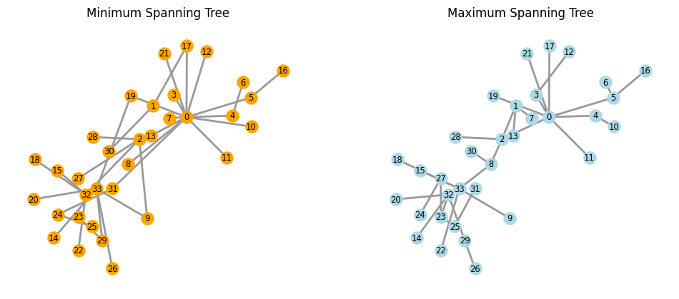
Maybe spanning trees are too fine

Are there other techniques that allow for more preservation of key important structure?

A sort of Goldilocks sparsification technique…?

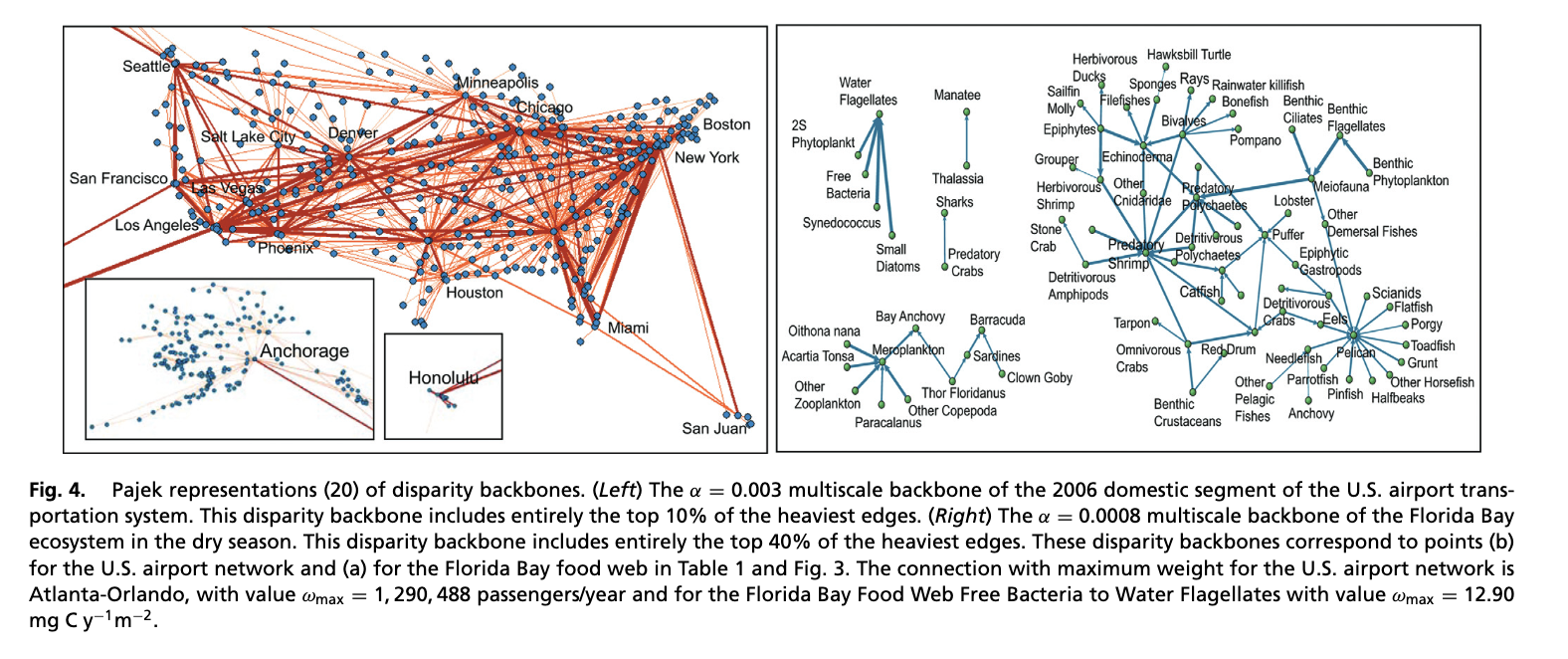
Entering: The Sparsification Wars ;)

tl;dr, there are a ton of ways to do this task, and many of them are effective! We’ll go over a few here and reference several others

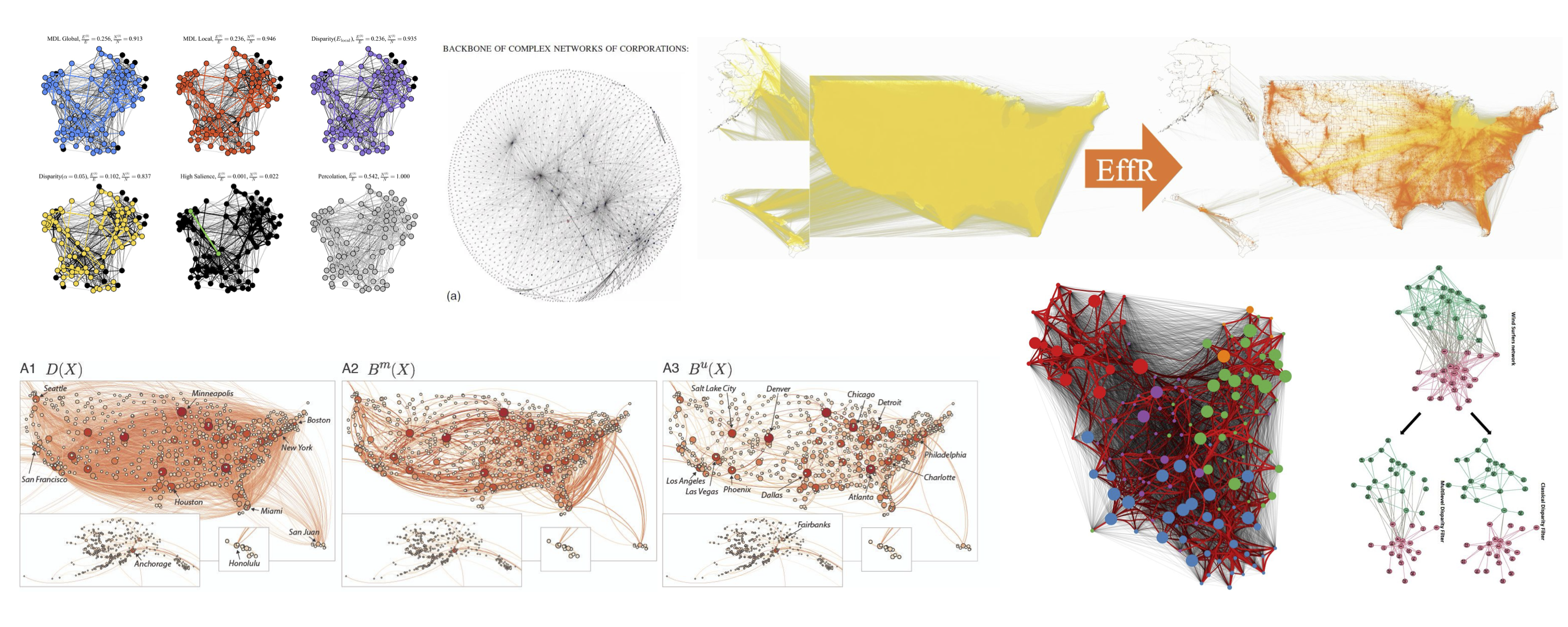
Image Sources:

• Kirkley, Alec. “Fast nonparametric inference of network backbones for weighted graph sparsification.” Physical Review X 15, no. 3 (2025): 031013.

• Glattfelder, J. B. (2012). Backbone of complex networks of corporations: The flow of control. In Decoding Complexity: Uncovering Patterns in Economic Networks (pp. 67-93). Berlin, Heidelberg: Springer Berlin Heidelberg.

• https://www.michelecoscia.com/?p=1236

• Mercier, A., Scarpino, S., & Moore, C. (2022). Effective resistance against pandemics: Mobility network sparsification for high-fidelity epidemic simulations. PLoS Computational Biology, 18(11).

• Simas, T., Correia, R.B., & Rocha, L.M.. The distance backbone of complex networks. Journal of Complex Networks, 9:cnab021, 2021.

• Hmaida, S., Cherifi, H., & El Hassouni, M. (2024). A multilevel backbone extraction framework. Applied Network Science, 9(1), 41.

---

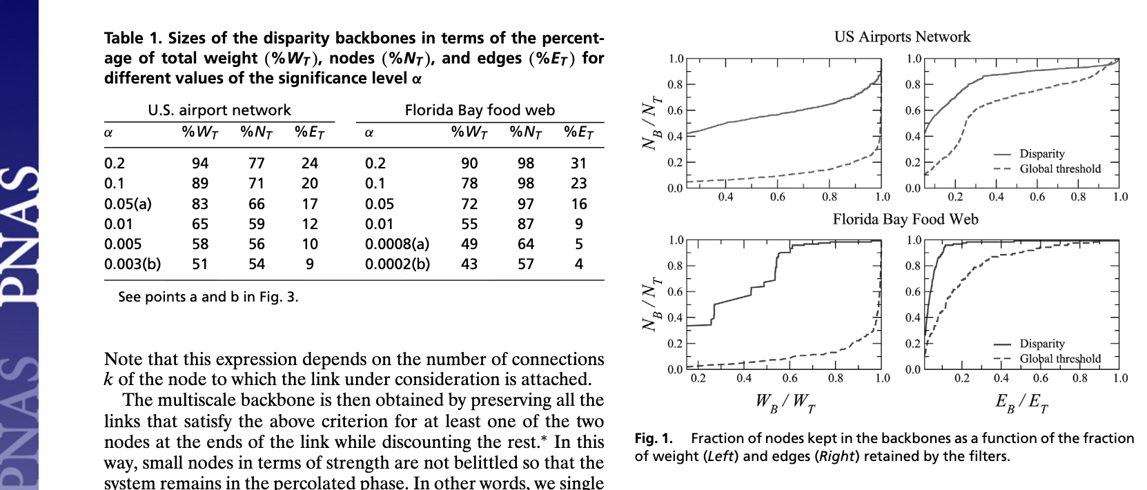
Sparsification Method: Disparity Filter

Global thresholding applies the same cutoff to all edges, regardless of how large or small a node’s total strength is. The disparity filter is a different approach: it uses a local null model at each node to identify edges whose weights are unexpectedly large compared to that node’s other connections.

The main idea is to preserve edges that carry a disproportionate fraction of a node’s strength, while discarding edges whose weight is compatible with a “random” allocation of strength. In this way, the disparity filter extracts a multi-scale backbone of dominant connections that respects the heterogeneity of the network and preserves structural hierarchies even when edge weights span several orders of magnitude.

Step 1: Normalizing edge weights

For a weighted, undirected graph, let \(s_i\) denote the strength of node \(i\) (the sum of weights of its incident edges), and let \(w_{ij}\) be the weight of edge \((i,j)\). The first step is to normalize each edge weight by the total strength of its incident node.

For each node \(i\) and neighbor \(j\) we define the normalized weight

\[ p_{ij} = \frac{w_{ij}}{s_i}, \]

so that

\[ \sum_{j \in N(i)} p_{ij} = 1. \]

Intuitively, \(p_{ij}\) is the fraction of \(i\)’s total strength that flows through edge \((i,j)\). Large values of \(p_{ij}\) indicate edges that dominate \(i\)’s connections.

Step 2: A local null model

Next we define a null model for how the normalized weights around a node might look if there were no particular preference for any neighbor.

For a node \(i\) with degree \(k_i\), the null model assumes that the unit interval \([0,1]\) is split into \(k_i\) segments by placing \(k_i-1\) cut points uniformly at random. The resulting segment lengths \( \{x_1, x_2, \dots, x_{k_i}\} \) represent the normalized weights \(\{p_{ij}\}\) under a purely random allocation of strength.

Under this null model, the probability density of a single normalized weight \(p\) is

\[ \rho(p) = (k_i - 1)(1 - p)^{k_i - 2}, \quad 0 \le p \le 1. \]

To assess whether an observed \(p_{ij}\) is unusually large for node \(i\), we compute the one-sided \(p\)-value: the probability that a random segment from this distribution is at least as large as \(p_{ij}\),

\[ \alpha_{ij} = \Pr\big(X \ge p_{ij}\big) = 1 - (k_i - 1)\int_0^{p_{ij}} (1 - x)^{k_i - 2}\,dx = (1 - p_{ij})^{k_i - 1}. \]

Small values of \(\alpha_{ij}\) mean that it is very unlikely, under the null model, to see a normalized weight as large as \(p_{ij}\) purely by chance.

Step 3: Choosing a significance level and defining the backbone

We now select a significance level \(\alpha\) (for example, \(\alpha = 0.05\)). For each edge \((i,j)\) we test the null model at each endpoint:

• compute \(\alpha_{ij}\) using node \(i\)’s degree and strength,

• compute \(\alpha_{ji}\) using node \(j\)’s degree and strength.

An edge is considered statistically significant for node \(i\) if

\[ \alpha_{ij} < \alpha,\]

and similarly for node \(j\). The edge \((i,j)\) is included in the backbone if it is significant for at least one of its endpoints.

---

A few details:

• Nodes with degree \(k_i = 1\) have no heterogeneity to test (there is only a single edge), so the null model is not very informative. In practice, the usual convention is:

  • if one endpoint has \(k > 1\) and the other has \(k = 1\), we only test significance using the endpoint with \(k > 1\);

  • edges between two degree-1 nodes can be kept or discarded by convention, since they do not affect local heterogeneity.

By construction, the disparity filter uses different effective thresholds for different nodes, depending on their degree and strength. This allows it to preserve significant edges of low-strength nodes (which would be wiped out by a global threshold) and to retain only the most dominant edges of high-degree, high-strength hubs.

def disparity_filter(G, alpha, weight_key="weight", copy_nodes=False):
    """
    Extract a disparity-filter backbone from a weighted, undirected graph.

    For each node n with degree k_n > 1, the function:
      1. Computes its strength
            s_n = sum_j w_{nj},
         where w_{nj} is the weight of edge (n, j).
      2. Computes normalized weights
            p_{nj} = w_{nj} / s_n.
      3. Evaluates the disparity-filter p-value
            alpha_{nj} = (1 - p_{nj})^(k_n - 1).
      4. If alpha_{nj} < alpha, the edge (n, j) is considered significant
         from n's perspective and is added to the backbone.

    Because we loop over all nodes, an undirected edge (i, j) can be added
    from either endpoint's perspective. In practice, this means edges that
    are significant for at least one endpoint are kept.

    Args:
        G: NetworkX graph. Assumed undirected, with positive edge weights.
        alpha: Significance level in (0, 1). Smaller alpha → sparser backbone.
        weight_key: Name of the edge attribute containing weights (default "weight").
        copy_nodes: If True, copy all nodes (and their attributes) from G
            into the backbone graph.

    Returns:
        keep_graph: A new NetworkX graph containing the backbone edges.
                    Node attributes (if copy_nodes=True) and edge attributes,
                    including weights, are preserved.
    """
    keep_graph = G.__class__()

    if copy_nodes:
        keep_graph.add_nodes_from(G.nodes(data=True))

    # Loop over all nodes in the original graph
    for n in G.nodes():
        neighbors = list(G[n])
        k_n = len(neighbors)

        # Nodes with degree <= 1 do not contribute to the disparity test
        if k_n <= 1:
            continue

        # Total strength s_n of node n
        sum_w = 0.0
        for nj in neighbors:
            sum_w += G[n][nj][weight_key]

        if sum_w <= 0:
            # If total strength is non-positive, skip this node
            continue

        # Examine each neighbor and test significance of the normalized weight
        for nj in neighbors:
            w_nj = G[n][nj][weight_key]
            p_nj = w_nj / sum_w  # normalized weight p_{nj}

            # Disparity-filter p-value: alpha_{nj} = (1 - p_{nj})^(k_n - 1)
            p_value = (1.0 - p_nj) ** (k_n - 1)

            # If p-value is below the chosen significance level, keep the edge
            if p_value < alpha:
                # Copy all edge attributes (including weight)
                edge_data = G[n][nj]
                keep_graph.add_edge(n, nj, **edge_data)

    return keep_graph

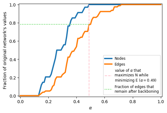
alphas = np.linspace(0,1,101)
G = nx.karate_club_graph()

N_vals = []
E_vals = []

for a in alphas:
    G_i = disparity_filter(G, a)
    N_vals.append(G_i.number_of_nodes()/\
                  G.number_of_nodes())
    E_vals.append(G_i.number_of_edges()/\
                  G.number_of_edges())
    

fig, ax = plt.subplots(1,1,figsize=(6,4),dpi=100)
ax.plot(alphas, N_vals, label='Nodes', lw=3)
ax.plot(alphas, E_vals, label='Edges', lw=3)

ideal_val_index = np.where(np.array(N_vals)==1.0)[0][0]
ax.vlines(alphas[ideal_val_index],0,1,color='pink',ls='--',
          label=r'value of $\alpha$ that'+'\nmaximizes N while'+'\nminimizing E '+\
                r'($\alpha=%.2f$)'%alphas[ideal_val_index])

ax.hlines(E_vals[ideal_val_index], 0, alphas[ideal_val_index], color='limegreen',
          ls=':', label='Fraction of edges that\nremain after backboning')

ax.legend(fontsize='small')
ax.set_xlabel(r'$\alpha$')
ax.set_ylabel("Fraction of original network's values")
ax.set_ylim(-0.01,1.01)
ax.set_xlim(-0.01,1.01)

plt.show()

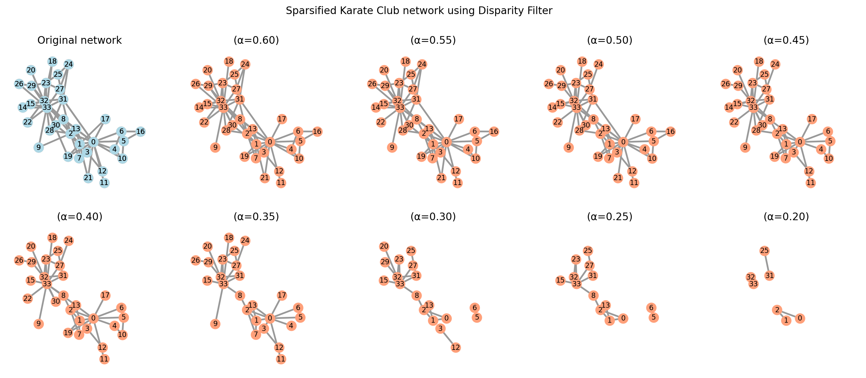
sparsified_graphs = {}
alphas = np.arange(0.2, 0.7, 0.05)

positions = nx.spring_layout(G, seed=3141592)

fig, axes = plt.subplots(2, 5, figsize=(18, 7), sharex=True, sharey=True, dpi=200) 

for i, alpha in enumerate(alphas):
    sparsified_graphs[alpha] = disparity_filter(G, alpha)
    
    nx.draw(sparsified_graphs[alpha], pos=positions, ax=axes.flat[-(i + 1)], 
            with_labels=True, node_color="lightsalmon", edge_color=".6", width=2,
            node_size=125, font_size='small')
    axes.flat[-(i + 1)].set_title(f"(α={alpha:.2f})")

# Original network
nx.draw(G, pos=positions, ax=axes.flat[0], with_labels=True, node_color="lightblue",
        edge_color=".6", width=2, node_size=125, font_size='small')
axes.flat[0].set_title("Original network")


plt.suptitle("Sparsified Karate Club network using Disparity Filter")


plt.show()

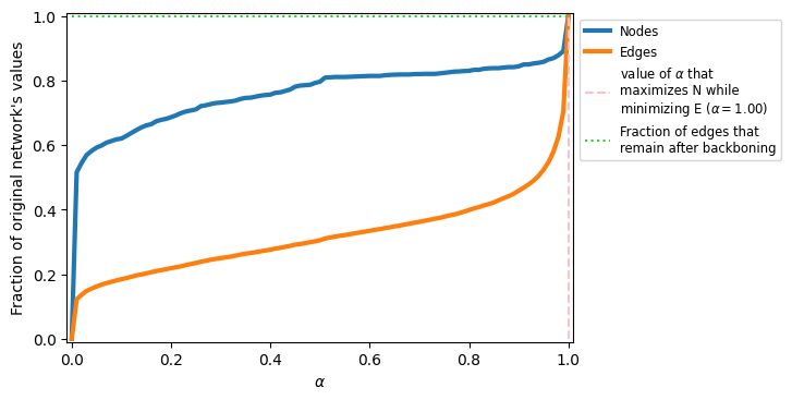
edges = pd.read_csv('data/openflights_USairport_2010.txt', sep=' ', header=None,
                    names=['source','target','weight'])
nodes = pd.read_csv('data/openflights_airports.txt', sep=' ')


w_edge_dict = dict(zip(list(zip(edges['source'],
                                edges['target'])), 
                       edges['weight']))

G = nx.Graph()
G.add_nodes_from(nodes['Airport ID'].values)
G.add_edges_from([(int(i),int(j),
                   {'weight':k})
                  for i,j,k in list(edges.values)])

Gx = nx.subgraph(G, max(nx.connected_components(G), key=len))

alphas = np.linspace(0,1,101)

N_vals = []
E_vals = []

for a in alphas:
    G_i = disparity_filter(Gx, a)
    N_vals.append(G_i.number_of_nodes()/\
                  Gx.number_of_nodes())
    E_vals.append(G_i.number_of_edges()/\
                  Gx.number_of_edges())

fig, ax = plt.subplots(1,1,figsize=(6,4),dpi=100)
ax.plot(alphas, N_vals, label='Nodes', lw=3)
ax.plot(alphas, E_vals, label='Edges', lw=3)

ideal_val_index = np.where(np.array(N_vals)==1.0)[0][0]
ax.vlines(alphas[ideal_val_index],0,1,color='pink',ls='--',
          label=r'value of $\alpha$ that'+'\nmaximizes N while'+'\nminimizing E '+\
                r'($\alpha=%.2f$)'%alphas[ideal_val_index])

ax.hlines(E_vals[ideal_val_index], 0, alphas[ideal_val_index], color='limegreen',
          ls=':', label='Fraction of edges that\nremain after backboning')

ax.legend(fontsize='small', loc=2, bbox_to_anchor=[1.0,1.0])
ax.set_xlabel(r'$\alpha$')
ax.set_ylabel("Fraction of original network's values")
ax.set_ylim(-0.01,1.01)
ax.set_xlim(-0.01,1.01)

plt.show()

---

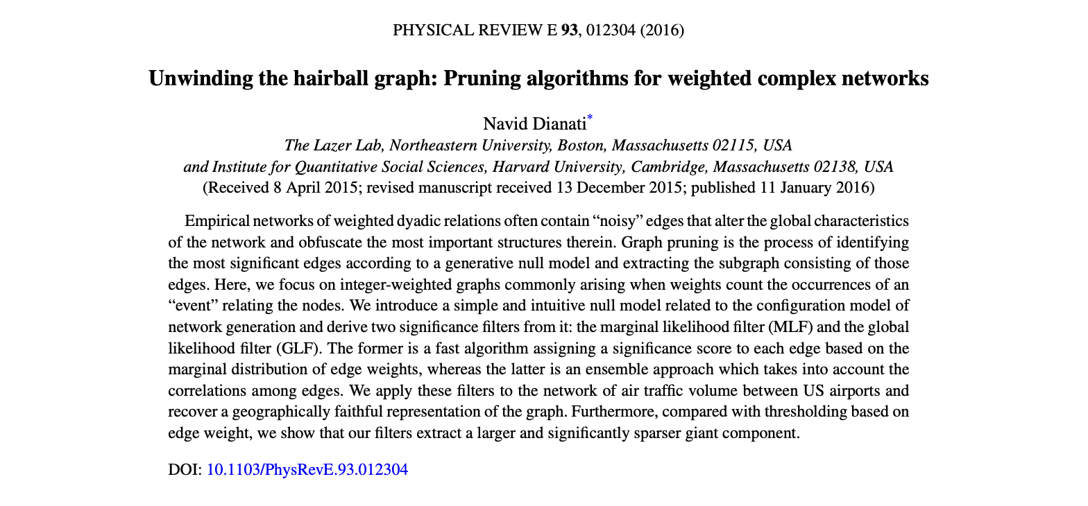
Sparsification Method: Marginal Likelihood Filter

The Marginal Likelihood Filter (MLF) is another statistical backbone extraction method for weighted networks. Whereas the disparity filter evaluates each edge from the local perspective of a single node, the MLF uses a global configuration model style null that depends on the strengths of both endpoints. This makes it more sensitive to edges that are unexpectedly strong given the strengths of the two nodes they connect.

Source: Dianati, N. (2016). Unwinding the hairball graph: Pruning algorithms for weighted complex networks. Physical Review E, 93(1), 012304. http://doi.org/10.1103/PhysRevE.93.012304

Mathematical framework for the MLF

Assume we have an undirected weighted graph where edge weights \(w_{ij}\) are non-negative integers counting discrete events (flights between airports, co-occurrences of words, etc.). Let \( s_i = \sum_j w_{ij} \) be the (integer) strength of node \(i\), and let \( T = \sum_{i<j} w_{ij} \) be the total number of unit edge contributions in the network.

The MLF null model imagines that these \(T\) unit contributions are assigned independently to unordered node pairs \((i,j)\), with probabilities proportional to the product of their strengths. Under this model, the probability that a single unit chooses the pair \((i,j)\) is

\[ p_{ij} = \frac{s_i s_j}{2 T^2},\]

so the total weight \(\sigma_{ij}\) realized on edge \((i,j)\) follows a binomial distribution

\[ \Pr\big[\sigma_{ij} = m \,\big|\, s_i, s_j, T\big] = \binom{T}{m} p_{ij}^{\,m}\, (1-p_{ij})^{T-m}, \qquad m = 0,1,\dots,T. \]

Given an observed edge weight \(w_{ij}\), the \(p\)–value under the null model is the probability of observing a value at least this large by chance:

\[ P(\sigma_{ij} \ge w_{ij}) = \sum_{m = w_{ij}}^{T} \binom{T}{m} p_{ij}^{\,m}\, (1-p_{ij})^{T-m} = 1 - \sum_{m = 0}^{w_{ij}-1} \binom{T}{m} p_{ij}^{\,m}\, (1-p_{ij})^{T-m}.\]

As with the disparity filter, we fix a significance level \(\alpha\) (for example, \(\alpha = 0.01\)) and retain edge \((i,j)\) in the backbone if \(P(\sigma_{ij} \ge w_{ij}) \le \alpha\).

Edges that pass this test are those whose observed weight is too large to be explained by the null model that redistributes \(T\) unit events at random proportional to node strengths. Because \(p_{ij}\) depends on both \(s_i\) and \(s_j\), the MLF can down-weight edges between very strong nodes (for which large weights are expected) and highlight unexpectedly strong ties involving weaker nodes.

from scipy.stats import binom

def marginal_likelihood_filter(G, alpha, weight_key="weight"):
    """
    Extract the backbone of a weighted, undirected network using the
    Marginal Likelihood Filter (MLF) of Dianati (2016).

    The method assumes integer edge weights w_ij representing counts of
    discrete events (e.g., flights, co-occurrences). Let

        s_i = sum_j w_ij          (strength of node i)
        T   = sum_{i<j} w_ij      (total number of unit edge contributions)

    Under the null model, each of the T unit contributions independently
    chooses an unordered pair (i, j) with probability

        p_ij = s_i * s_j / (2 * T^2),

    so the realized edge weight sigma_ij follows a Binomial(T, p_ij)
    distribution. For each observed edge (i, j) with weight w_ij, the
    p-value is

        p_value = P(sigma_ij >= w_ij)
                = 1 - BinomCDF(w_ij - 1; T, p_ij).

    The backbone keeps only those edges whose p-value is at most alpha.

    Parameters
    ----------
    G : networkx.Graph
        Undirected weighted graph. Edge weights should be non-negative
        integers stored under `weight_key`.
    alpha : float
        Significance level (0 < alpha < 1). Smaller values yield sparser
        backbones.
    weight_key : str, optional
        Name of the edge attribute containing integer weights
        (default: "weight").

    Returns
    -------
    backbone : networkx.Graph
        A graph containing only the edges that pass the Marginal Likelihood
        Filter at the given significance level. Node attributes are copied
        from G, and edge weights are preserved.
    """
    if G.is_directed():
        raise ValueError("marginal_likelihood_filter assumes an undirected graph.")

    # New graph for the backbone; preserve graph type and node attributes
    backbone = G.__class__()
    backbone.add_nodes_from(G.nodes(data=True))

    # Compute node strengths and total weight T = sum_{i<j} w_ij
    strengths = {node: 0.0 for node in G.nodes()}
    T = 0.0

    for u, v, data in G.edges(data=True):
        w_uv = data.get(weight_key, 0.0)
        if w_uv <= 0:
            continue
        strengths[u] += w_uv
        strengths[v] += w_uv
        T += w_uv

    if T <= 0:
        # No positive weights, nothing to do
        return backbone

    # For each edge, compute its binomial p-value under the null model
    for u, v, data in G.edges(data=True):
        w_uv = data.get(weight_key, 0.0)
        if w_uv <= 0:
            continue

        s_u = strengths[u]
        s_v = strengths[v]

        # Edge probability under the null:
        # p_ij = s_i * s_j / (2 * T^2)
        p_ij = (s_u * s_v) / (2.0 * T**2)

        # Numerical safety: clamp p_ij to [0, 1]
        p_ij = max(0.0, min(1.0, p_ij))

        # p-value: P(sigma_ij >= w_uv) = 1 - CDF(w_uv - 1)
        # Note: binom.cdf(k, n, p) = P(X <= k)
        p_value = 1.0 - binom.cdf(w_uv - 1, int(T), p_ij)

        if p_value <= alpha:
            backbone.add_edge(u, v, **data)

    return backbone

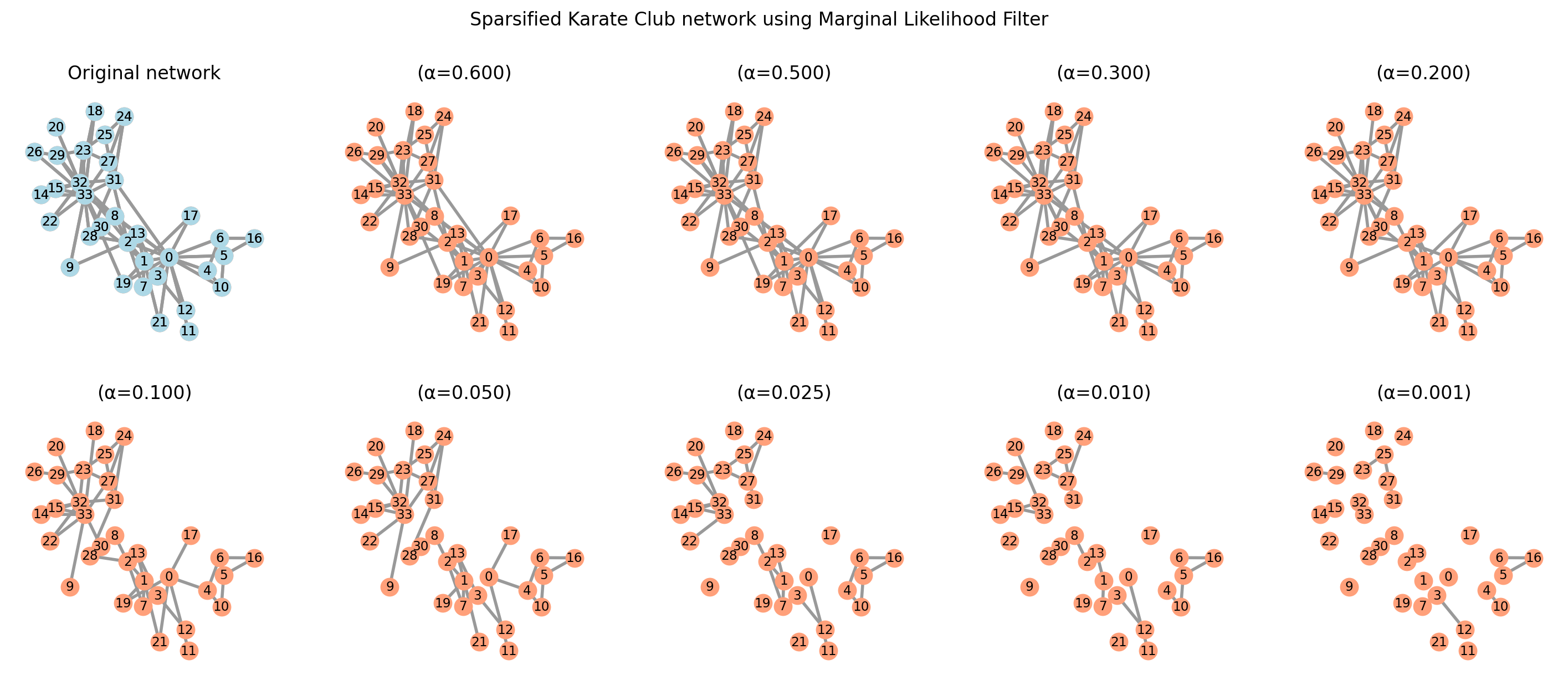
G = nx.karate_club_graph()

sparsified_graphs = {}
alphas = [0.001, 0.01, 0.025, 0.05, 0.1, 0.2, 0.3, 0.5, 0.6, 0.7]

positions = nx.spring_layout(G, seed=3141592)

fig, axes = plt.subplots(2, 5, figsize=(18, 7), sharex=True, sharey=True, dpi=200) 

for i, alpha in enumerate(alphas[:10]):
    sparsified_graphs[alpha] = marginal_likelihood_filter(G, alpha)

    nx.draw(sparsified_graphs[alpha], pos=positions,  ax=axes.flat[-(i + 1)], 
            with_labels=True, node_color="lightsalmon", edge_color=".6", width=2,
            node_size=125, font_size='small')
    axes.flat[-(i + 1)].set_title(f"(α={alpha:.3f})")

# Original network
nx.draw(G, pos=positions, ax=axes.flat[0], with_labels=True, node_color="lightblue",
        node_size=125, font_size='small', edge_color=".6", width=2)


axes.flat[0].set_title("Original network")
plt.suptitle("Sparsified Karate Club network using Marginal Likelihood Filter")


plt.show()

Evaluation techniques and applications

Evaluating the performance of backbone extraction methods is essential to ensure their reliability and appropriateness for specific tasks. Below, we will cover t a set of criteria and metrics that can be used to assess the performance of these methods.

US domestic flights traffic data 2021-2022

In this section, we will use the domestic nonstop segment of the U.S. airport transportation system for the interval 2021-2022, which can be downloaded from here.

df = pd.read_table("data/db28seg.dd.wac.2021.2022.asc", sep="|", low_memory=False)
df

	year	month	origin	origin_city_market_id	origin_wac	origin_city_name	dest	dest_city_market_id	dest_wac	dest_city_name	...	departures_scheduled	payload	seats	passengers	freight	mail	ramp_to_ramp	air_time	Wac	Unnamed: 28
0	2021	5	01A	30001	1	Afognak Lake, AK	A43	30056	1	Kodiak Island, AK	...	0	1200	6	1	0	0	20	18	1	NaN
1	2021	8	01A	30001	1	Afognak Lake, AK	A43	30056	1	Kodiak Island, AK	...	0	750	5	1	0	0	30	28	1	NaN
2	2022	8	01A	30001	1	Afognak Lake, AK	A43	30056	1	Kodiak Island, AK	...	0	2400	12	7	0	0	47	43	1	NaN
3	2021	8	01A	30001	1	Afognak Lake, AK	A43	30056	1	Kodiak Island, AK	...	0	2400	12	2	0	0	43	39	1	NaN
4	2021	9	01A	30001	1	Afognak Lake, AK	A43	30056	1	Kodiak Island, AK	...	0	6000	30	0	0	0	105	95	1	NaN
...	...	...	...	...	...	...	...	...	...	...	...	...	...	...	...	...	...	...	...	...	...
787386	2021	4	ZXU	36353	15	North Kingstown, RI	TEB	35167	21	Teterboro, NJ	...	0	3450	8	1	0	0	72	54	10	NaN
787387	2021	12	ZXU	36353	15	North Kingstown, RI	TEB	35167	21	Teterboro, NJ	...	0	3450	8	1	0	0	54	36	10	NaN
787388	2022	12	ZXU	36353	15	North Kingstown, RI	TEB	35167	21	Teterboro, NJ	...	0	3450	8	1	0	0	54	42	10	NaN
787389	2021	9	ZXU	36353	15	North Kingstown, RI	TEB	35167	21	Teterboro, NJ	...	0	3450	8	1	0	0	54	42	10	NaN
787390	2021	4	ZZV	36361	44	Zanesville, OH	SAT	33214	74	San Antonio, TX	...	0	2500	8	3	0	0	202	194	54	NaN

787391 rows × 29 columns

print("Number of unique origin airports", len(df["origin"].unique()))
print("Number of unique destination airports", len(df["dest"].unique()))
print()
print("Columns:", [column for column in df.columns])

Number of unique origin airports 1547
Number of unique destination airports 1544

Columns: ['year', 'month', 'origin', 'origin_city_market_id', 'origin_wac', 'origin_city_name', 'dest', 'dest_city_market_id', 'dest_wac', 'dest_city_name', 'Carrier', 'Carrier_Entity', 'carrier_group', 'distance', 'Svc_Class', 'Aircraft_Group', 'Aircraft_type', 'Aircraft_Config', 'departures_performed', 'departures_scheduled', 'payload', 'seats', 'passengers', 'freight', 'mail', 'ramp_to_ramp', 'air_time', 'Wac', 'Unnamed: 28']

df["route"] = df.apply(lambda row: tuple(sorted([row["origin"], row["dest"]])), axis=1)
edges = df.groupby("route")["passengers"].sum().reset_index()
edges[["airport_1", "airport_2"]] = pd.DataFrame(edges["route"].tolist(), index=edges.index)
edges = edges.drop(columns=["route"])
edges = edges.loc[edges["passengers"] > 0]
edges = edges.loc[edges["airport_1"] != edges["airport_2"]]
edges.sort_values(by="passengers", ascending=False)

	passengers	airport_1	airport_2
20617	4823868	JFK	LAX
3523	4774008	ATL	MCO
3458	4467829	ATL	FLL
21518	4326505	LAS	LAX
12428	4181994	DEN	PHX
...	...	...	...
7273	1	BOS	MQY
20918	1	KCQ	ORI
6399	1	BKG	BTL
1714	1	AGN	EXI
26220	1	PAE	SUN

20607 rows × 3 columns

Now, in order to produce some nice visualizations, nothing better than use the real coordinates of each airport. However, this is contained on a separate dataset, can also be downloaded here [7].

unique_airports = pd.concat([edges["airport_1"], edges["airport_2"]]).unique()
print("Number of unique airports", len(unique_airports))
airport_coords = pd.read_csv("data/airport_coords.csv")
airport_coords = airport_coords[airport_coords["AIRPORT"].isin(unique_airports)].drop_duplicates(subset="AIRPORT", keep="first")
airport_coords

Number of unique airports 1501

	AIRPORT_SEQ_ID	AIRPORT_ID	AIRPORT	DISPLAY_AIRPORT_NAME	DISPLAY_AIRPORT_CITY_NAME_FULL	AIRPORT_WAC	AIRPORT_COUNTRY_NAME	AIRPORT_COUNTRY_CODE_ISO	AIRPORT_STATE_NAME	AIRPORT_STATE_CODE	...	LATITUDE	LON_DEGREES	LON_HEMISPHERE	LON_MINUTES	LON_SECONDS	LONGITUDE	AIRPORT_START_DATE	AIRPORT_THRU_DATE	AIRPORT_IS_CLOSED	AIRPORT_IS_LATEST
0	1000101	10001	01A	Afognak Lake Airport	Afognak Lake, AK	1	United States	US	Alaska	AK	...	58.109444	152.0	W	54.0	24.0	-152.906667	7/1/2007 12:00:00 AM	NaN	0	1
3	1000501	10005	05A	Little Squaw Airport	Little Squaw, AK	1	United States	US	Alaska	AK	...	67.570000	148.0	W	11.0	2.0	-148.183889	8/1/2007 12:00:00 AM	NaN	0	1
4	1000601	10006	06A	Kizhuyak Bay	Kizhuyak, AK	1	United States	US	Alaska	AK	...	57.745278	152.0	W	52.0	58.0	-152.882778	10/1/2007 12:00:00 AM	NaN	0	1
7	1000901	10009	09A	Augustin Island	Homer, AK	1	United States	US	Alaska	AK	...	59.362778	153.0	W	25.0	50.0	-153.430556	6/1/2008 12:00:00 AM	NaN	0	1
8	1001001	10010	1B1	Columbia County	Hudson, NY	22	United States	US	New York	NY	...	42.288889	73.0	W	42.0	37.0	-73.710278	4/1/2009 12:00:00 AM	6/30/2011 12:00:00 AM	0	0
...	...	...	...	...	...	...	...	...	...	...	...	...	...	...	...	...	...	...	...	...	...
19991	1697401	16974	MD3	Harford County	Churchville, MD	35	United States	US	Maryland	MD	...	39.566944	76.0	W	12.0	9.0	-76.202500	6/1/2022 12:00:00 AM	9/30/2022 12:00:00 AM	0	0
19996	1697601	16976	MLJ	Baldwin County Regional	Milledgeville, GA	34	United States	US	Georgia	GA	...	33.154167	83.0	W	14.0	29.0	-83.241389	6/1/2022 12:00:00 AM	NaN	0	1
20000	1697901	16979	MS6	Columbia Marion County	Columbia, MS	53	United States	US	Mississippi	MS	...	31.297778	89.0	W	48.0	41.0	-89.811389	7/1/2022 12:00:00 AM	NaN	0	1
20004	1698201	16982	2AK	Deer Park	Deerpark, AK	1	United States	US	Alaska	AK	...	56.519722	134.0	W	40.0	46.0	-134.679444	6/1/2021 12:00:00 AM	6/30/2025 12:00:00 AM	1	1
20007	1698501	16985	A9K	Era Denali Heliport	Healy, AK	1	United States	US	Alaska	AK	...	63.738333	148.0	W	52.0	54.0	-148.881667	1/1/2021 12:00:00 AM	6/30/2025 12:00:00 AM	0	0

1500 rows × 28 columns

airport_network = nx.Graph()
for _, row in edges.iterrows():
    airport_network.add_edge(row['airport_1'], row['airport_2'], weight=row['passengers'])
airport_network.remove_node("DQG") # No coordinates for this airport

print("Number of nodes", len(airport_network))
print("Number of edges", len(airport_network.edges))

Number of nodes 1500
Number of edges 20598

pos  = airport_coords.set_index('AIRPORT')[['LONGITUDE', 'LATITUDE']].apply(tuple, axis=1).to_dict()

fig, ax = plt.subplots(1,1,figsize=(7,5),dpi=100)

node_strength = {node: sum(weight for _, _, weight in airport_network.edges(node, data="weight"))
                 for node in airport_network.nodes}
node_sizes = np.array([2 + 0.05 * np.sqrt(node_strength[node]) for node in airport_network.nodes])/2
node_colors = [np.log10(node_strength[node]) for node in airport_network.nodes]
edge_weights = [np.log10(airport_network[u][v]["weight"]) for u, v in airport_network.edges]

nx.draw_networkx_nodes(airport_network, pos=pos, node_color=node_colors, 
                       node_size=node_sizes, cmap=plt.cm.viridis, ax=ax)

nx.draw_networkx_edges(airport_network, pos=pos, alpha=0.3, edge_color=".6", ax=ax)


ax.set_xlabel("Longitude", fontsize=12)
ax.set_ylabel("Latitude", fontsize=12)
ax.set_xlim(-180, -60) 
ax.set_ylim(15, 75) 


plt.show()

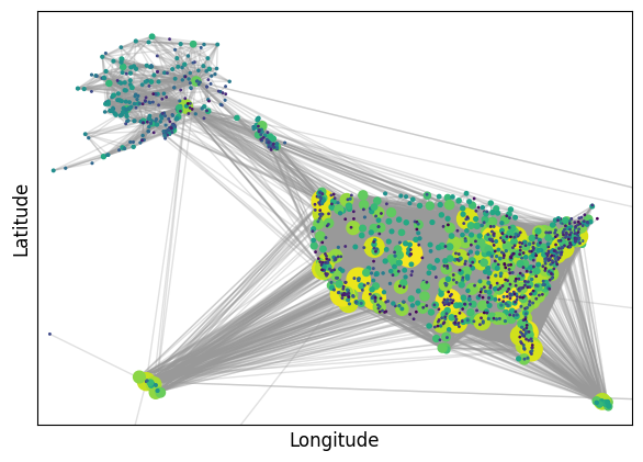
As we can see, the visualization is not very informative. We can observer some hubs, but it is not possible to observer any useful details. Now, let’s try with a sparsified version.

fig, axes = plt.subplots(2, 3, figsize=(17,8), sharex=True, sharey=True, dpi=200)
plt.subplots_adjust(wspace=0.1)

func_names = ["Global Threshold", "Disparity Filter", "Marginal Likelihood Filter",
              'Minimum Spanning Tree', "Maximum Spanning Tree"]
backbone_functions = [threshold_graph, disparity_filter, marginal_likelihood_filter,
                      nx.maximum_spanning_tree, nx.minimum_spanning_tree, ]
parameters = [200000, 0.001, 0.000001, 'kruskal', 'kruskal']
sparsified_networks = []

for i, func in enumerate(backbone_functions):
    airport_network_sparsified = func(airport_network, parameters[i])
    sparsified_networks.append(airport_network_sparsified)
    
    node_strength = {node: sum(weight for _, _, weight in airport_network_sparsified.edges(node, data="weight"))
                     for node in airport_network_sparsified.nodes}
    node_sizes = np.array([2 + 0.02 * np.sqrt(node_strength[node]) for node in airport_network_sparsified.nodes])/2
    node_colors = [np.log10(node_strength[node]) for node in airport_network_sparsified.nodes]

    nx.draw_networkx_nodes(airport_network_sparsified, pos=pos, node_color=node_colors,
                           node_size=node_sizes, cmap=plt.cm.viridis, ax=axes.flat[i])
    
    nx.draw_networkx_edges(airport_network_sparsified, pos=pos, alpha=0.2, 
                           edge_color=".6", ax=axes.flat[i])

    axes.flat[i].set_title(func_names[i])
    axes.flat[i].set_xlim(-180, -60)
    axes.flat[i].set_ylim(15, 75)


plt.savefig('images/pngs/compare_filters.png', dpi=425, bbox_inches='tight')
plt.savefig('images/pdfs/compare_filters.pdf', dpi=425, bbox_inches='tight')
plt.show()

<ipython-input-34-84a10d480fe8>:18: RuntimeWarning: divide by zero encountered in log10
  node_colors = [np.log10(node_strength[node]) for node in airport_network_sparsified.nodes]

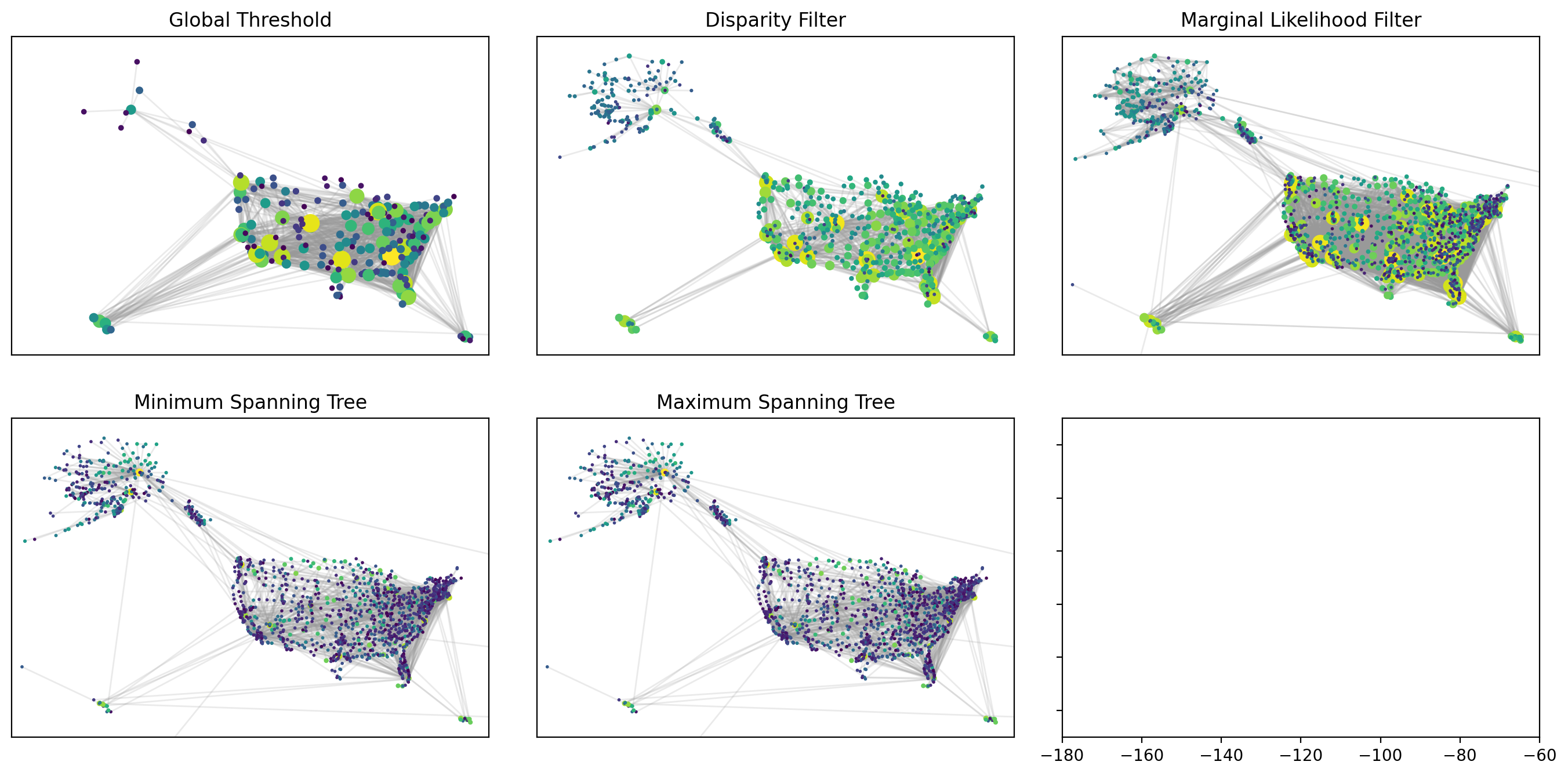
How to evaluate sparsification techniques?

So far, we have extracted different backbones for the U.S. domestic flights from 2021 to 2022. How can we evaluate the quality of each backbone? First, what we mean by quality will depend on our interests. For example, if we just care about having a nice visualization, we could that the backbones extracted using Disparity Filter and Maximum Spanning Tree are better than the other two. If we care about having connectivity, we could assert that MST is the best one. There are different things we could use as an evaluation metric to compare different backbones of a single network.

We can separate metrics intro three groups, where we measure: topological properties, topological properties distributions, and dynamics. In this notebook, we will mainly focus on topological properties.

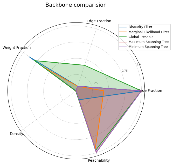
Topological properties

The simplest way of evaluating a backbone is by comparing different topological properties. Here, we select node fraction, edge fraction, weight fraction, _average degree, density, and reachability.

(If there’s time) Your Turn!

Implement a function that computes the topological properties mentioned above for a list of backbones, and create a nice visualization of it.

def topological_properties(graph, original_graph):
    """
    Compute topological properties of a graph compared to the original graph.

    Parameters:
        graph (networkx.Graph): The backbone graph to evaluate.
        original_graph (networkx.Graph): The original graph to compare against.

    Returns:
        dict: A dictionary containing the following metrics:
            - Node Fraction: Fraction of nodes retained in the backbone.
            - Edge Fraction: Fraction of edges retained in the backbone.
            - Weight Fraction: Fraction of total edge weight retained in the backbone.
            - Average Degree: Average degree of nodes in the backbone.
            - Density: Density of the backbone.
            - Reachability: Fraction of nodes in the largest connected component.
    """
    
    pass
    
#     return metrics

---

def topological_properties(graphs, original_graph):
    """
    Compute topological properties for a list of graphs compared to the original graph.

    Parameters:
        graphs (list of networkx.Graph): List of backbone graphs to evaluate.
        original_graph (networkx.Graph): The original graph to compare against.

    Returns:
        list of dict: A list of dictionaries containing the following metrics for each graph:
            - Node Fraction: Fraction of nodes retained in the backbone.
            - Edge Fraction: Fraction of edges retained in the backbone.
            - Weight Fraction: Fraction of total edge weight retained in the backbone.
            - Average Degree: Average degree of nodes in the backbone.
            - Density: Density of the backbone.
            - Reachability: Fraction of nodes in the largest connected component.
    """
    metrics_list = []
    for graph in graphs:
        metrics = {}
        metrics["Node Fraction"] = graph.number_of_nodes() / original_graph.number_of_nodes()
        metrics["Edge Fraction"] = graph.number_of_edges() / original_graph.number_of_edges()
        total_weight_original = sum(weight for _, _, weight in original_graph.edges(data="weight", default=1))
        total_weight_backbone = sum(weight for _, _, weight in graph.edges(data="weight", default=1))
        metrics["Weight Fraction"] = total_weight_backbone / total_weight_original
        #metrics["Average Degree"] = np.mean([deg for _, deg in graph.degree()])
        metrics["Density"] = nx.density(graph)
        largest_cc = max(nx.connected_components(graph), key=len)
        metrics["Reachability"] = len(largest_cc) / graph.number_of_nodes()
        metrics_list.append(metrics)
    return metrics_list

def radar_chart(metrics_list, labels, title):
    """
    Create an improved radar chart to visualize multiple metrics across different backbones.

    Parameters:
        metrics_list (list of dict): List of dictionaries containing metrics for each backbone.
        labels (list of str): Labels for each backbone.
        title (str): Title of the radar chart.

    Returns:
        None
    """
    categories = list(metrics_list[0].keys())
    num_vars = len(categories)
    angles = np.linspace(0, 2 * np.pi, num_vars, endpoint=False).tolist()
    angles += angles[:1]
    fig, ax = plt.subplots(figsize=(8, 7), subplot_kw={"polar": True}, dpi=100)
    for metrics, label in zip(metrics_list, labels):
        values = list(metrics.values())
        values += values[:1]
        ax.plot(angles, values, label=label, linewidth=2)
        ax.fill(angles, values, alpha=0.25)
    ax.set_yticks([0.25, 0.5, 0.75, 1.0])
    ax.set_yticklabels(["0.25", "0.5", "0.75", "1.0"], color="gray", size=8)
    ax.set_xticks(angles[:-1])
    ax.set_xticklabels(categories, fontsize=10)
    ax.set_title(title, size=15, y=1.1)
    ax.grid(color="gray", linestyle="--", linewidth=0.5, alpha=0.7)
    ax.legend(loc="upper right", bbox_to_anchor=(1.2, 1), fontsize=9)
#     sns.set_style("whitegrid")
#     plt.tight_layout()
    plt.show()

metrics_list = topological_properties(sparsified_networks, airport_network)
labels = ["Disparity Filter", "Marginal Likelihood Filter", "Global Treshold",
          "Maximum Spanning Tree", 'Minimum Spanning Tree']
radar_chart(metrics_list, labels, "Backbone comparision")

Conclusion

Large and complex networks often present significant challenges. The sheer number of nodes and edges can make them difficult to analyze, computationally expensive to process, and hard to interpret visually. This is where network sparsification becomes a valuable tool. By simplifying networks and keeping only the most important connections, we can make our work much more efficient and focused, while still preserving the key information we need.

The main lesson here is that each method serves a specific purpose, and choosing the right one depends on your goal. Do you want a clearer visualization? Do you need to preserve connectivity? Or are you looking to make computations faster? Sparsification offers tools to meet these needs, and experimenting is an essential item in the network scientist toolkit in order to find the best approach.

We recommend consulting documentation for the netbone Python library, which implements all the techniques covered in this notebook, as well a many more state-of-the-art backbone extraction methods. Also, it offers a complete evaluation framework.

Source: Yassin, A., Haidar, A., Cherifi, H., Seba, H., & Togni, O. (2023). An evaluation tool for backbone extraction techniques in weighted complex networks. Scientific Reports, 13(1), 17000. https://www.nature.com/articles/s41598-023-42076-3

---

Next time…

Network Sampling class_22_sampling.ipynb

---

References and further resources:

1. Class Webpages

   • Jupyter Book: https://network-science-data-and-models.github.io/phys7332_fa25/README.html

   • Github: https://github.com/network-science-data-and-models/phys7332_fa25/

   • Syllabus and course details: https://brennanklein.com/phys7332-fall25

2. Alvarez-Hamelin, J. I., Dall’Asta, L., Barrat, A., & Vespignani, A. (2005). k-core decomposition: A tool for the visualization of large scale networks. https://hal.science/hal-00004807v2/file/k-cores_AHDVB_v2.pdf

3. Bonanno, G., Caldarelli, G., Lillo, F., & Mantegna, R. N. (2003). Topology of correlation-based minimal spanning trees in real and model markets. Physical Review E, 68(4), 046130. https://doi.org/10.1103/PhysRevE.68.046130

4. Daqing, L., Kosmidis, K., Bunde, A., & Havlin, S. (2011). Dimension of spatially embedded networks. Nature Physics, 7(6), 481-484. https://www.nature.com/articles/nphys1932

5. Graham, R. L., & Hell, P. (1985). On the history of the minimum spanning tree problem. Annals of the History of Computing, 7(1), 43-57. http://doi.org/10.1109/MAHC.1985.10011

6. Radicchi, F., Ramasco, J. J., & Fortunato, S. (2011). Information filtering in complex weighted networks. Physical Review E, 83(4), 046101. http://doi.org/10.1103/PhysRevE.83.046101

7. Seidman, S. B. (1983). Network structure and minimum degree. Social Networks, 5(3), 269-287. http://doi.org/10.1016/0378-8733(83)90028-X

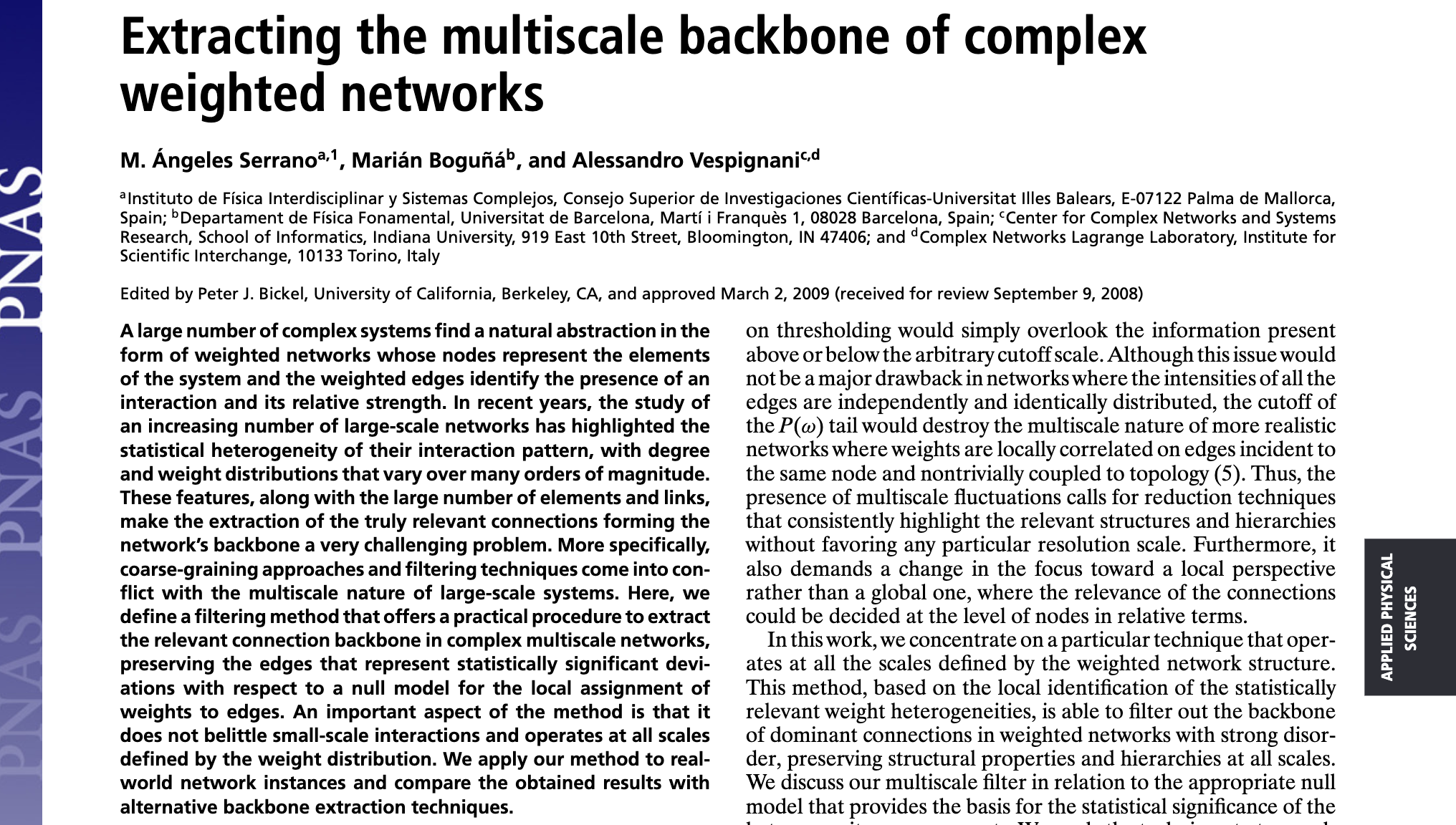
8. Serrano, M. Á., Boguná, M., & Vespignani, A. (2009). Extracting the multiscale backbone of complex weighted networks. Proceedings of the National Academy of Sciences, 106(16), 6483-6488. https://www.pnas.org/doi/10.1073/pnas.0808904106

9. Tumminello, M., Aste, T., Di Matteo, T., & Mantegna, R. N. (2005). A tool for filtering information in complex systems. Proceedings of the National Academy of Sciences, 102(30), 10421-10426. https://doi.org/10.1073/pnas.0500298102

10. Spielman, D. A., & Srivastava, N. (2011). Graph sparsification by effective resistances. SIAM Journal on Computing, 40(6), 1913–1926. https://doi.org/10.1137/080734029

11. Benczúr, A. A., & Karger, D. R. (2015). Randomized approximation schemes for cuts and flows in capacitated graphs. SIAM Journal on Computing, 44(2), 290–319. https://doi.org/10.1137/070705970

12. Hamann, M., Lindner, G., Meyerhenke, H., Staudt, C. L., & Wagner, D. (2016). Structure-preserving sparsification methods for social networks. Social Network Analysis and Mining, 6, 23. https://arxiv.org/abs/1601.00286

13. Dianati, N. (2016). Unwinding the hairball graph: Pruning algorithms for weighted complex networks. Physical Review E, 93(1), 012304. https://doi.org/10.1103/PhysRevE.93.012304

14. Mercier, A., Scarpino, S., & Moore, C. (2022). Effective resistance against pandemics: Mobility network sparsification for high-fidelity epidemic simulations. PLoS Computational Biology, 18(11). https://doi.org/10.1371/journal.pcbi.1010650

15. Neal, Z. (2014). The backbone of bipartite projections: Inferring relationships from co-authorship, co-sponsorship, co-attendance and other co-behaviors. Social Networks, 39, 84–97. https://doi.org/10.1016/j.socnet.2014.06.001

16. Simas, T., Correia, R.B., & Rocha, L.M.. The distance backbone of complex networks. Journal of Complex Networks, 9:cnab021, 2021. https://doi.org/10.1093/comnet/cnab021.

17. Yassin, A., Haidar, A., Cherifi, H., Seba, H., & Togni, O. (2023). An evaluation tool for backbone extraction techniques in weighted complex networks. Scientific Reports, 13(1), 17000. https://www.nature.com/articles/s41598-023-42076-3