Class 22: Network Sampling#
Goal of today’s class:
Define what network sampling means in theory and practice
Introduce biases that emerge when sampling networks
Highlight several key sampling approaches
Acknowledgement: This lesson is based on material created by Matteo Chinazzi and Qian Zhang in a previous version of this course.
Come in. Sit down. Open Teams.
Find your notebook in your /Class_22/ folder.
import networkx as nx
import numpy as np
import matplotlib.pyplot as plt
from matplotlib import rc
rc('axes', axisbelow=True)
rc('axes', fc='w')
rc('figure', fc='w')
rc('savefig', fc='w')
Why sample networks?#
Up to now in the course we’ve mostly treated the network as if it were “the” system: someone hands us an adjacency matrix or an edge list, and our job is to analyze it. In almost every real application, though, that observed graph is itself the product of a sampling process. We only see some people and not others, some interactions and not others, some parts of the infrastructure and not others. Thinking carefully about how a network was sampled—and about whether we want to intentionally sample it differently—is central to making valid inferences from network data.
There are at least three broad reasons why sampling is unavoidable:
Many networks are too large, dynamic, or restricted to observe in full. Online social networks, the Web, or Internet router-level topologies are measured through APIs, logs, and traceroute-like probes that capture only a subset of nodes and links. Internet mapping projects, for example, send probes from a limited set of sources to many destinations and reconstruct a router-level map from the union of those paths; by construction this is a sampled view of the underlying topology, and it can be heavily biased toward high-degree routers and frequently used routes.
Classic work on traceroute sampling shows that even if the underlying network is relatively homogeneous, the sampled view can look much more heavy-tailed or hierarchical than it really is. In neuroscience, we often record activity from a small subset of neurons or brain regions and treat that as a proxy for the full functional connectivity network. In transportation and mobility, we might see only trips from a subset of apps, cell towers, or ticketing systems, and infer a larger mobility network from partial traces.
Second, even when a full network exists somewhere, practical constraints often force intentional subsampling. Large social, information, or biological networks can contain millions or billions of nodes and edges; storing and processing the full graph may be prohibitively expensive, especially in streaming or online settings. This has motivated a large literature on graph sampling for data mining: selecting a smaller subgraph that approximately preserves degree distributions, clustering, community structure, motif counts, or distances, so that downstream algorithms can run on the sample instead of the full network.
Work on sampling from large graphs shows that different sampling schemes (node-based, edge-based, exploration-based) vary in how well they preserve statistics like diameter, degree distribution, and clustering, and introduces ideas like scaled-down or coarse-grained graphs (match a smaller network) or back-in-time graphs (match an earlier snapshot of a growing graph). More recent papers extend this to streaming settings, where the graph is observed as a sequence of edges and the sampling algorithm has strict memory and one-pass constraints.
Third, in many domains the only way to collect data at all is through link-tracing or chain-referral sampling. Hidden or hard-to-reach populations—such as people who inject drugs, sex workers, or some migrant communities—are often studied through snowball or respondent-driven sampling, where participants recruit their contacts into the study. Here, the network is not just a sampling application; the mechanism behind the network itself is a walk or branching process on the social network, and the dependence structure of the sample paths strongly affects estimators.
Methods like Network Sampling with Memory explicitly exploit network structure and respondents’ local knowledge to reduce design effects and improve efficiency. Similar link-tracing designs appear in epidemiological contact tracing (following chains of infection), and in measurements of online social networks, where API rate limits or platform restrictions force us to crawl along edges rather than enumerate all nodes.
Some common sampling procedures:
Induced subgraph sampling (sample nodes uniformly, keep all edges between them),
Incident (or ego-centered) subgraph sampling (sample nodes and keep edges incident to them),
Snowball / link-tracing sampling (start from seeds and iteratively add neighbors),
Random-walk sampling (move step by step along edges according to a Markov chain),
More advanced algorithms such as random walks with jumps, Metropolis-Hastings walks, or noise-corrected topological sampling for online social networks.
Network Sampling Formalism#
To formalize this, it helps to imagine a (usually unobserved) population graph \(G = (V, E)\) and an observed sampled graph \(G_s = (V_s, E_s)\). Under a given sampling approach, each node \(i \in V\) has some inclusion probability \(\pi_i\), and each edge \(e_{ij} \in E\) has an inclusion probability \(\pi_{ij}\). A central theme in the theory papers on network sampling is: when do the distributions of key statistics in \(G_s\) belong to the same “family” as in \(G\)? For example, work on subgraphs of scale-free networks and on the statistical properties of sampled networks shows that:
even if the full network has a clean power-law degree distribution, many common sampling schemes produce samples that are not scale-free, or that have apparent exponents very different from the truth;
different sampling strategies (random node sampling, degree-biased sampling, BFS-like exploration, etc.) can systematically distort degree distributions, assortativity, path lengths, betweenness, and clustering in different ways.
A descriptor of the graph \(G\) is denoted by \(\Phi (G)\) (remember Chapter 19 on Graph Distances). \(\Phi (G)\) can be a point statistic such as the average degree of the nodes in \(V\) or the global clustering coefficient of the graph, or a distribution such as the degree distribution or the clustering distribution, etc.
In other words, many familiar network statistics—degree, clustering, centrality, community structure—can be dramatically distorted by the sampling method. Different approaches produce systematically different views of the same underlying graph. This matters not just for descriptive analysis, but also for inference and comparison: for example, comparing two large networks via sub-sampling strategies, or training a classifier on sampled networks and asking whether performance reflects the underlying topology or the sampling artifacts.
In this chapter we will lean into this perspective: instead of treating the adjacency matrix as a given object, we will treat the observed network as the output of a sampling design applied to some (usually unknown) underlying graph. We will look at several common designs—node-based, edge-based, and topology-based samplers—and see how each one selects different parts of the graph, how it biases standard network statistics, and how we can sometimes correct for those biases. The goal is not to turn everyone into a survey statistician, but to make it hard to look at a network dataset again without asking: what sampling process produced this graph, and what does that imply for the conclusions I’m about to draw?
To start class: A challenge!#
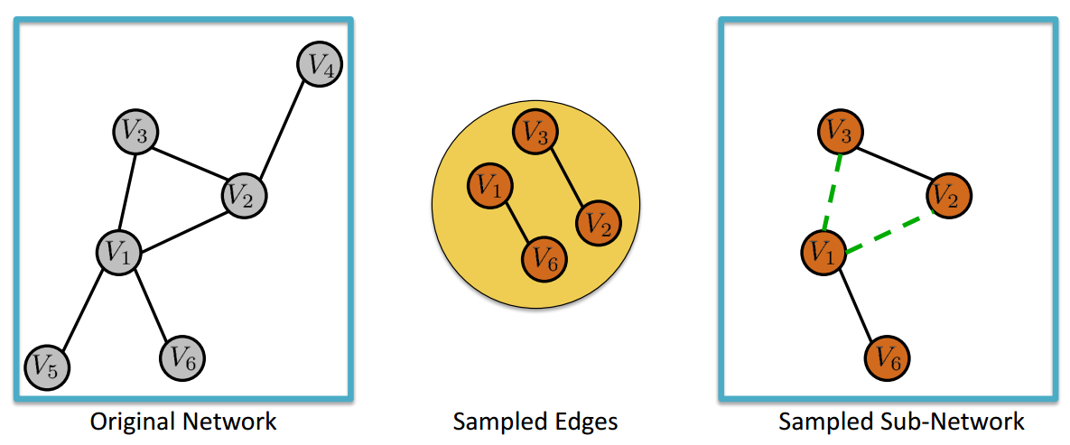
In 2005, an influential (and short) paper was published, showing that subgraphs of scale-free networks are not necessarily scale-free.
Source: Stumpf, M. P., Wiuf, C., & May, R. M. (2005). Subnets of scale-free networks are not scale-free: sampling properties of networks. Proceedings of the National Academy of Sciences, 102(12), 4221-4224. https://www.pnas.org/doi/full/10.1073/pnas.0501179102
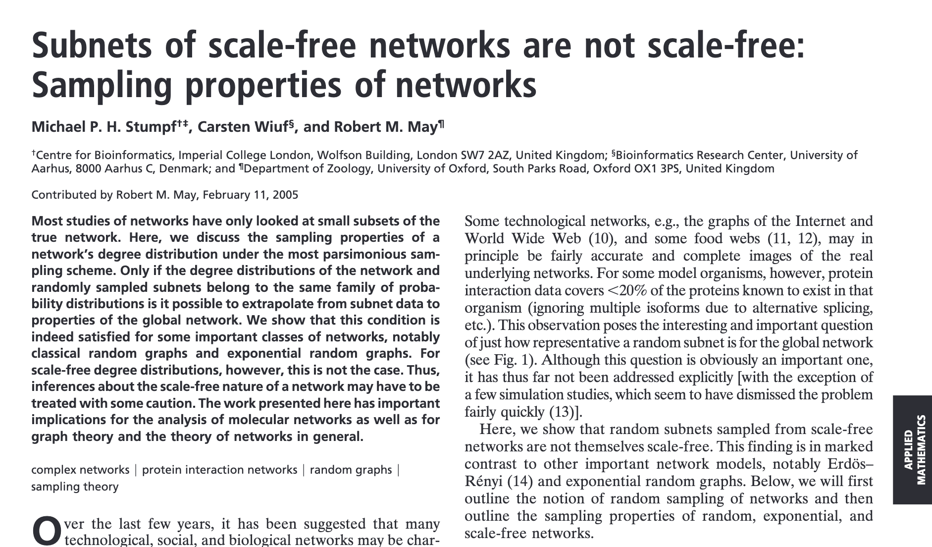
The authors used the following sampling procedure (left), and showed that randomly sampling a (e.g.) Barabasi-Albert graph at \(p=0.2\) and \(p=0.8\) densities produces degree distributions that appear not to be scale-free.
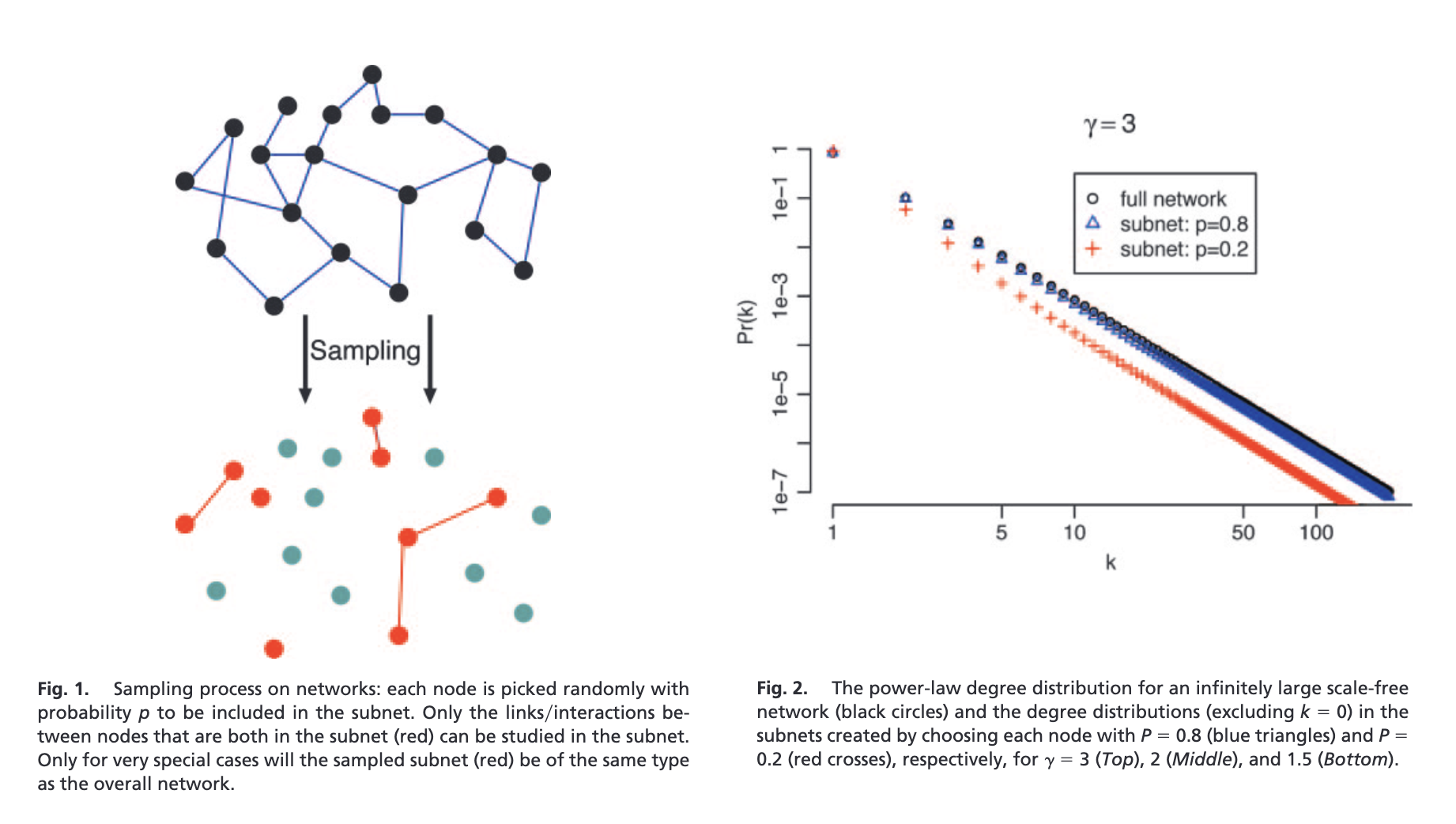
Let’s reproduce this result, in stages. What ingredients do we need to reproduce this figure?
pass
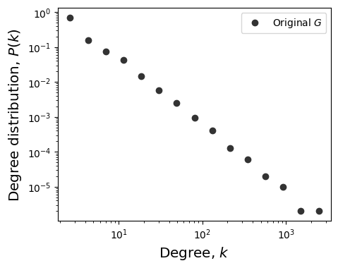
Generate a BA network (of large enough size to observe the finding)
Measure and plot its degree distribution
Create a sampling algorithm, according to Fig. 1 above
Sample a graph, G_s, from G, based on \(p=0.2\) of the nodes
Plot the degree distribution G_s
# 1.
N = 1_000_000
m = 2

G = nx.barabasi_albert_graph(N, m)
def get_binning(data, num_bins=40, is_pmf=False, log_binning=False, threshold=0):
    """
    Bins the input data and calculates the probability mass function (PMF) or
    probability density function (PDF) over the bins. Supports both linear and
    logarithmic binning.

    Parameters
    ----------
    data : array-like
        The data to be binned, typically a list or numpy array of values.
    num_bins : int, optional
        The number of bins to use for binning the data (default is 15).
    is_pmf : bool, optional
        If True, computes the probability mass function (PMF) by normalizing
        histogram counts to sum to 1. If False, computes the probability density
        function (PDF) by normalizing the density of the bins (default is True).
    log_binning : bool, optional
        If True, uses logarithmic binning with log-spaced bins. If False, uses
        linear binning (default is False).
    threshold : float, optional
        Only values greater than `threshold` will be included in the binning,
        allowing for the removal of isolated nodes or outliers (default is 0).

    Returns
    -------
    x : numpy.ndarray
        The bin centers, adjusted to be the midpoint of each bin.
    p : numpy.ndarray
        The computed PMF or PDF values for each bin.

    Notes
    -----
    This function removes values below a specified threshold, then defines
    bin edges based on the specified binning method (linear or logarithmic).
    It calculates either the PMF or PDF based on `is_pmf`.
    """

    # Filter out isolated nodes or low values by removing data below threshold
    values = list(filter(lambda x: x > threshold, data))
#     if len(values) != len(data):
#         print("%s isolated nodes have been removed" % (len(data) - len(values)))

    # Define the range for binning (support of the distribution)
    lower_bound = min(values)
    upper_bound = max(values)

    # Define bin edges based on binning type (logarithmic or linear)
    if log_binning:
        # Use log-spaced bins by taking the log of the bounds
        lower_bound = np.log10(lower_bound)
        upper_bound = np.log10(upper_bound)
        bin_edges = np.logspace(lower_bound, upper_bound, num_bins + 1, base=10)
    else:
        # Use linearly spaced bins
        bin_edges = np.linspace(lower_bound, upper_bound, num_bins + 1)

    # Calculate histogram based on chosen binning method
    if is_pmf:
        # Calculate PMF: normalized counts of data in each bin
        y, _ = np.histogram(values, bins=bin_edges, density=False)
        p = y / y.sum()  # Normalize to get probabilities
    else:
        # Calculate PDF: normalized density of data in each bin
        p, _ = np.histogram(values, bins=bin_edges, density=True)

    # Compute bin centers (midpoints) to represent each bin
    x = bin_edges[1:] - np.diff(bin_edges) / 2  # Bin centers for plotting

    # Remove bins with zero probability to avoid plotting/display issues
    x = x[p > 0]
    p = p[p > 0]

    return x, p
# 2. Plot degree distribution of G
fig, ax = plt.subplots(1,1,figsize=(5,4),dpi=100)
plt.subplots_adjust(wspace=0.25)

x, y = get_binning(list(dict(G.degree()).values()),
                   num_bins=15, log_binning=True, is_pmf=True)

ax.loglog(x,y,'o',color='.2', label=r'Original $G$')
ax.set_ylabel(r'Degree distribution, $P(k)$',fontsize='x-large')
ax.set_xlabel(r'Degree, $k$',fontsize='x-large')

# p = 0.2
# G_s02 = sample_subgraph_random_nodes(G, p, seed=9)
# x_s02, y_s02 = get_binning(list(dict(G_s02.degree()).values()),
#                    num_bins=15, log_binning=True, is_pmf=True)

# ax.loglog(x_s02,y_s02,'s',color='palevioletred', label=r'$G_s$ (p=0.2)',mec='.9')

# p = 0.8
# G_s08 = sample_subgraph_random_nodes(G, p, seed=9)
# x_s08, y_s08 = get_binning(list(dict(G_s08.degree()).values()),
#                    num_bins=15, log_binning=True, is_pmf=True)

# ax.loglog(x_s08,y_s08,'s',color='crimson', label=r'$G_s$ (p=0.8)',mec='.9')


ax.legend()


plt.show()
Your turn: Create a function to create G_s as described in Fig. 1 above#
# 3. YOUR TURN!

def sample_subgraph_random_nodes(G, p=0.2):
    """
    Random node sampling:
      - keep each node independently with probability p
      - return the induced subgraph on the kept nodes, G_s
    """

    pass


    return G_s
pass
you have 5 minutes
def sample_subgraph_random_nodes(G, p, seed=None):
    """
    Random node sampling:
      - keep each node independently with probability p
      - return the induced subgraph on the kept nodes
    """
    rng = np.random.default_rng(seed)
    nodes = [n for n in G.nodes if rng.random() < p]
    return G.subgraph(nodes).copy()
# 2. Plot degree distribution of G
fig, ax = plt.subplots(1,1,figsize=(5,4),dpi=100)
plt.subplots_adjust(wspace=0.25)

x, y = get_binning(list(dict(G.degree()).values()),
                   num_bins=15, log_binning=True, is_pmf=True)

ax.loglog(x,y,'o',color='.2', label=r'Original $G$ ($\gamma=3$)')
ax.set_ylabel(r'Degree distribution, $P(k)$',fontsize='x-large')
ax.set_xlabel(r'Degree, $k$',fontsize='x-large')

p = 0.2
G_s02 = sample_subgraph_random_nodes(G, p, seed=9)
x_s02, y_s02 = get_binning(list(dict(G_s02.degree()).values()),
                   num_bins=15, log_binning=True, is_pmf=True)

ax.loglog(x_s02,y_s02,'s',color='palevioletred', label=r'$G_s$ (p=0.2)',mec='.9')

p = 0.8
G_s08 = sample_subgraph_random_nodes(G, p, seed=9)
x_s08, y_s08 = get_binning(list(dict(G_s08.degree()).values()),
                   num_bins=15, log_binning=True, is_pmf=True)

ax.loglog(x_s08,y_s08,'s',color='crimson', label=r'$G_s$ (p=0.8)',mec='.9')


ax.legend()


plt.show()
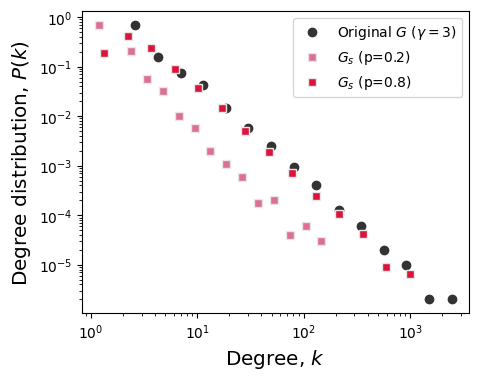
Still to do, on your own time: Measure the degree exponent of \(G_s\)
Classes of Sampling Methods#
Node Selection: a subset of nodes is sampled;
Edge Selection: a subset of edges is sampled;
Topology-based Sampling (exploration sampling): the topology of the population graph is used to extract the sampled graph.
Final note: a lot of the motivation behind this chapter comes from the (phenomenal) book, specifically Chapter 5:
Kolaczyk, E. D. (2009). Sampling and estimation in network graphs. In Statistical Analysis of Network Data: Methods and Models (pp. 1-30). New York, NY: Springer New York. https://link.springer.com/book/10.1007/978-0-387-88146-1
Method 1: Induced Subgraph Sampling#
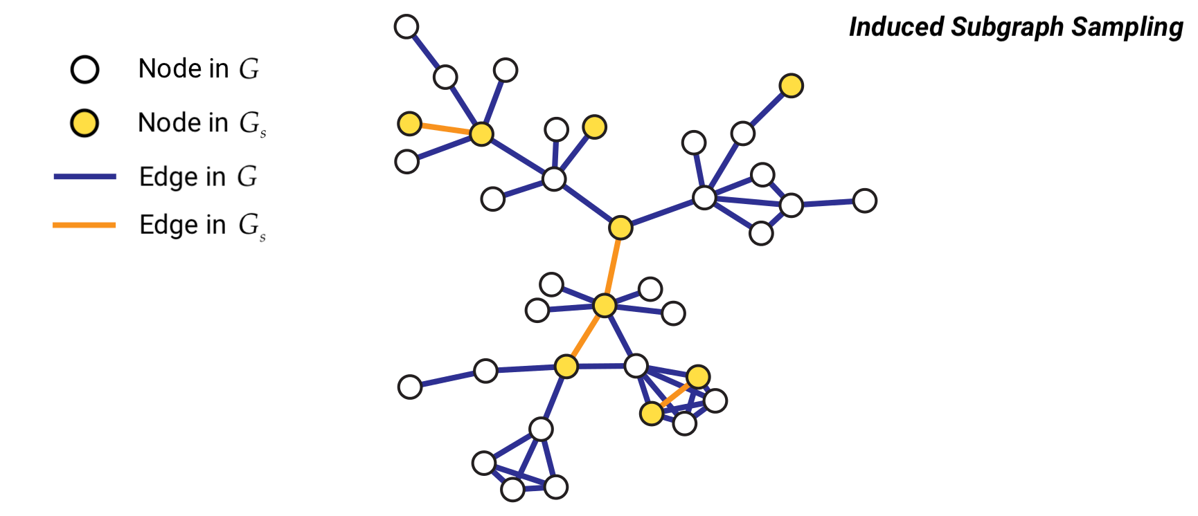
Induced subgraph sampling consists in drawing at random \(n\) vertices from a graph of size \(N\). In particular, let us denote with \(G = (V,E)\) the original graph and with \(G_s = (V_s,E_s)\) the sampled subgraph. Then, the set \(V_s\) includes the \(n\) nodes randomly drawn from \(V\) and \(E_s\) contains all the edges \(e_{i,j}\) such that both \(i\) and \(j\) belong to \(V_s\).
In this case, the vertex inclusion probability is equal to \(\pi_i = \frac{n}{N};\) while the edge inclusion probability is equal to \( \pi_{e_{i,j}} = \frac{n(n-1)}{N(N-1)}\), \(\forall i \in V\), and \(\forall e_{i,j} \in E\).
Vertex inclusion probability - proof#
Given that our sample size is \(n\), we can extract up to \(\binom{N}{n}\) different samples if we do not impose any contraint on whether or not a specific node is selected. However, if we do impose that node \(i\) has to be included, then the total number of possible samples becomes \(\binom{N-1}{n-1}\).
Therefore, the vertex inclusion probability of a generic node \(i\) is:
N = 1000
M = 50000
average_degree = 2*M/N
print(average_degree)

p = average_degree/(N-1)
G_er = nx.erdos_renyi_graph(N,p)
G_ws = nx.watts_strogatz_graph(N, int(average_degree), p=0.01)

print("Average degree ER:", np.mean(list(dict(G_er.degree()).values())))
print("Average degree WS:",  np.mean(list(dict(G_ws.degree()).values())))
100.0
Average degree ER: 99.928
Average degree WS: 100.0
from numpy.random import choice
def induced_subgraph_sampling(G, n):
    """
    Samples an induced subgraph of `n` nodes from the input graph `G`.

    Parameters
    ----------
    G : networkx.Graph
        The input graph from which the subgraph is sampled.
    n : int
        The number of nodes to include in the sampled induced subgraph.

    Returns
    -------
    subgraph : networkx.Graph
        The induced subgraph with `n` nodes and the edges among them.

    Raises
    ------
    ValueError
        If `n` is larger than the number of nodes in the graph.
    """
    # Ensure `n` is not larger than the number of nodes in G
    if n > G.number_of_nodes():
        raise ValueError("`n` must be less than or equal to the number of nodes in the graph.")

    # Get the list of nodes in the graph
    nodes = list(G.nodes())

    # Randomly sample `n` nodes without replacement
    sampled_nodes = np.random.choice(nodes, size=n, replace=False)

    # Create an induced subgraph of G using the sampled nodes
    subgraph = G.subgraph(sampled_nodes).copy()

    return subgraph
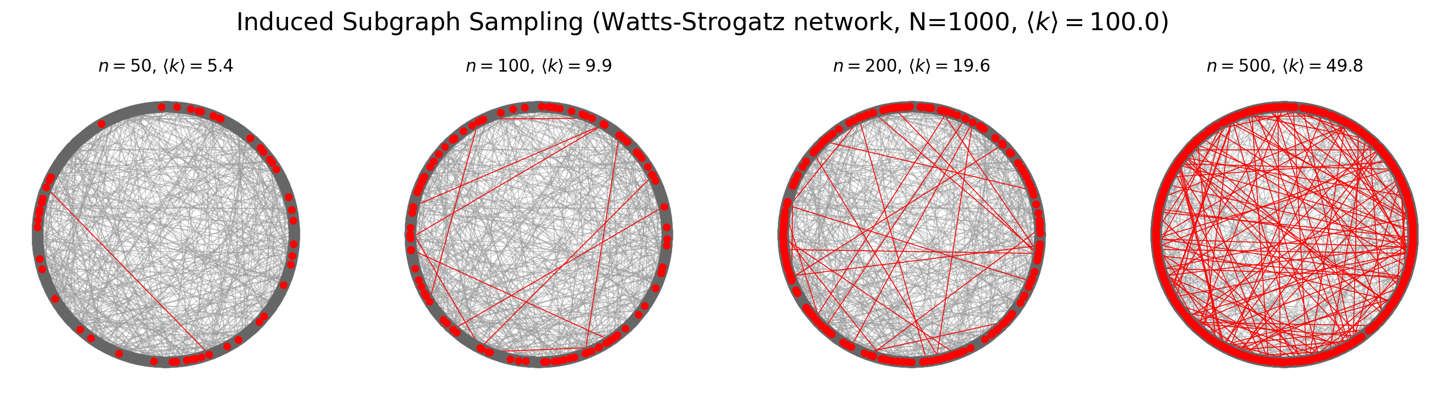
pos = nx.circular_layout(G_ws)
fig, ax = plt.subplots(1,4,figsize=(18,4),dpi=200)

for ni,n in enumerate([50,100,200,500]):
    subg = induced_subgraph_sampling(G_ws, n)
    nx.draw(G_ws, pos, node_color='.4', node_size=50, alpha=0.5, edge_color='.6', width=0.6, ax=ax[ni])
    nx.draw(subg, pos, node_color='red',node_size=20, edge_color='red', width=0.6, ax=ax[ni])
    ax[ni].set_title(r'$n = %i$, $\langle k \rangle = %.1f$'%(n, np.mean(list(dict(subg.degree).values()))))

plt.suptitle(r'Induced Subgraph Sampling (Watts-Strogatz network, N=%i, $\langle k \rangle = %.1f$)'%(
    G_ws.number_of_nodes(),average_degree),
             y=1.05, fontsize='xx-large')
plt.show()
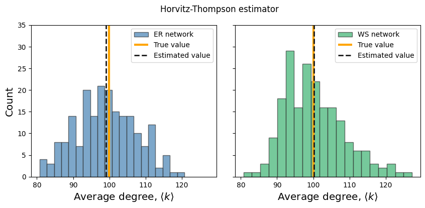
Statistics note: The Horvitz-Thompson Estimator#
Let \(U\) be a population of size \(N\) (e.g. Facebook users, Twitter users, etc..) and let \(y_i\) be a variable of interest associated to each individual \(i\) in the population \(U\) (e.g. number of friends, number of followers, etc..). Let us denote with \(\tau\) the total and with \(\mu\) the average of the \(y_i\)’s values, i.e. \(\tau = \sum_i y_i\) and \(\mu = \tau/N\). Let us also denote with \(S\) a sample of \(n\) units from population \(N\) and assume that for each unit \(i\) in sample \(S\) we observe the value \(y_i\). Then, we can use the Horvitz-Thompson estimator to estimate the value of \(\tau\) and \(\mu\) from the random sample \(S\):
where \(\pi_{i}\) denotes the inclusion probability of unit \(i\) in the sample \(S\).
Estimate the average degree of the graph from the sampled graph#
To estimate \(M\) we can use the Horvitz-Thompson estimator:
Our individual \(i\) is the edge \(e_{i,j}\)
The total we want to estimate is: \(\tau = M = \sum_i y_i = \sum_{e_{i,j}}1\)
In our case, the edge inclusion probability is: \( \pi_{e_{i,j}} = \frac{n(n-1)}{N(N-1)} ,\)
Therefore we can estimate \(\hat{M}\) as: \( \hat{\tau}_\pi = \sum_{e_{i,j} \in S} \frac{1}{\pi_{e_{i,j}}} = M_s\frac{N(N-1)}{n(n-1)}\)
Then, we can compute \(\hat{k}\) as: \(\hat{k} = \frac{2\hat{M}}{N}\).
fig, ax = plt.subplots(1,2,figsize=(10,4),dpi=100,sharey=True,sharex=True)
plt.subplots_adjust(wspace=0.1)
cols = ['steelblue','mediumseagreen']

B = 200 # number of simulations
labels = ['ER','WS']
for a, G in enumerate([G_er, G_ws]):
    av_degs = np.zeros(B)
    for b in range(B):
        n = 50
        subg_G = induced_subgraph_sampling(G, n)
        m = subg_G.number_of_edges()
        prob_e = n*(n-1)/N/(N-1)
        M_est = m/prob_e
        av_degs[b] = 2*M_est/N


    ax[a].hist(av_degs, 20, label=labels[a]+" network", color=cols[a], ec='.2', alpha=0.7)
    degs_G = np.mean(list(dict(G.degree()).values()))
    ax[a].vlines(degs_G, 0, 35, lw=3, label='True value', color='orange')

    mu = np.mean(av_degs)
    ax[a].vlines(mu, 0, 35, color='.1', lw=2, label='Estimated value', ls='--')
    ax[a].legend()
    ax[a].set_ylim(0,35)
    ax[a].set_xlabel(r'Average degree, $\langle k \rangle$', fontsize='x-large')

ax[0].set_ylabel('Count', fontsize='x-large')

plt.suptitle('Horvitz-Thompson estimator')

plt.show()
Estimation of Group Size#
To estimate the number of nodes of a graph from a sampled graph we can use the following capture-recapture estimator:
We sample two distinct graphs using the induced subgraph sampling design and we denote the number of nodes in the two graphs with \(n_1\) and \(n_2\), respectively;
We count the number of nodes that the two sampled graphs have in common (we denote this number with \(n_c\));
We estimate the number of nodes in the original graph using the estimator \( \hat{N} = \frac{n_1 n_2}{n_c}\).
B = 2500  # Number of iterations
N = 1000  # True size of the network

nodes = list(range(N))

# Array to store network size estimates
N_est = np.zeros(B)

### Perform capture-recapture simulation
for b in range(B):
    # Randomly sample the size of the first and second sample sets
    n1 = np.random.randint(150, 200)
    n2 = np.random.randint(150, 200)

    # Randomly select nodes for the first and second samples
    V_s1 = np.random.choice(nodes, size=n1, replace=False)
    V_s2 = np.random.choice(nodes, size=n2, replace=False)

    # Count the number of nodes in the intersection (recaptured nodes)
    n_c = len(set(V_s1).intersection(V_s2))

    # Estimate the network size if recaptured nodes exist; otherwise, set to NaN
    N_est[b] = n1 * n2 / n_c if n_c > 0 else np.nan


# Filter out invalid estimates (NaN values)
N_est = N_est[np.isfinite(N_est)]

#################

fig, ax = plt.subplots(1, 1, figsize=(9, 4), dpi=100)
ax.hist(N_est, bins=50, color='.8', edgecolor='.2', alpha=0.7)
# ax.set_yticks(range(0,25,5))
ax.set_ylim(0)
ylims = ax.get_ylim()

ax.vlines(N, 0, ylims[1]*1.2, linewidth=3, label='True value', color='orange')

mu = np.mean(N_est)
ax.vlines(mu, 0, ylims[1]*1.2, color='.1', linewidth=2, label='Estimated value', linestyle='--')

ax.set_ylim(0, ylims[1]*1.2)
ax.legend()
ax.set_ylabel('Count',fontsize='x-large')
ax.set_xlabel(r'Network size, $N$',fontsize='x-large')


plt.show()
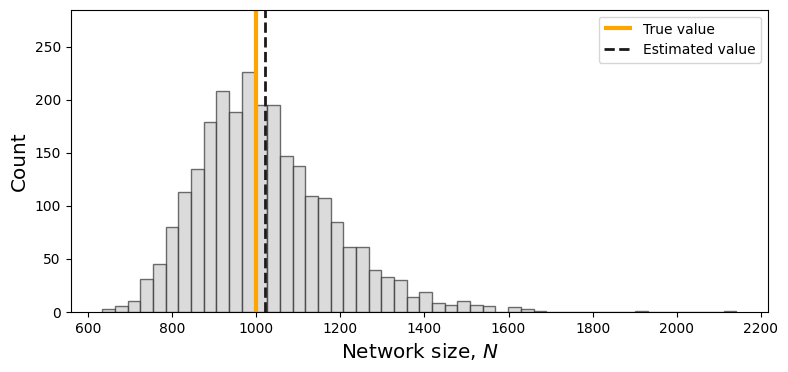
(That is very cool!)
N = 10000

frac = [0.001, 0.01, 0.05, 0.1, 0.2]
n_iter = 100
for f in frac:
    est = []
    for _ in range(n_iter):
        n1 = int(np.random.normal(f*N, 2))
        n2 = int(np.random.normal(f*N, 2))

        sample1 = np.random.choice(list(range(N)), n1, replace=False)
        sample2 = np.random.choice(list(range(N)), n2, replace=False)

        est.append(len(set(sample1).intersection(sample2)))

    print("frac =",f, "\tsampled set size = %.2f"%np.mean(est), "\tnetwork size estimate = %.2f"%(n1*n2/np.mean(est)))
<ipython-input-17-349beb88ca1d>:16: RuntimeWarning: divide by zero encountered in double_scalars
  print("frac =",f, "\tsampled set size = %.2f"%np.mean(est), "\tnetwork size estimate = %.2f"%(n1*n2/np.mean(est)))
frac = 0.001 	sampled set size = 0.00 	network size estimate = inf
frac = 0.01 	sampled set size = 0.87 	network size estimate = 11724.14
frac = 0.05 	sampled set size = 25.35 	network size estimate = 9802.84
frac = 0.1 	sampled set size = 101.32 	network size estimate = 9919.07
frac = 0.2 	sampled set size = 400.30 	network size estimate = 9987.51
Method 2: Incident Subgraph Sampling#
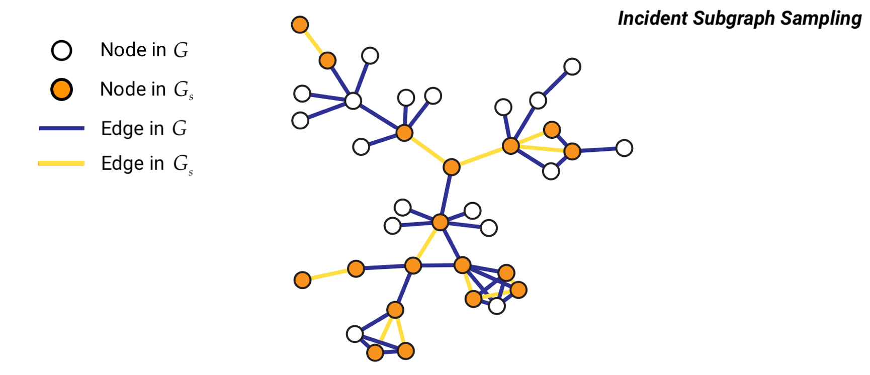
Incident subgraph sampling involves drawing \(n\) edges at random from a graph of size \(N\). Let us denote with \(G = (V,E)\) the original graph and with \(G_s = (V_s,E_s)\) the sampled subgraph. Then, the set \(E_s\) includes the \(n\) edges randomly selected from \(E\) and \(V_s\) contains all the nodes incident to the selected edges such that \(\forall e_{i,j} \in E_s\), \(i,j \in V_s\).
In this case, the vertex inclusion probability is equal to:
while the edge inclusion probability is equal to:
\(\forall i \in V\), and \(\forall e_{i,j} \in E\).
Notice that \(\pi_i\) is computed as one minus the probability of not sampling an edge incident to \(i\).
from random import shuffle

def incident_subgraph_sampling(G, n, is_directed=False):
    """
    Samples an incident subgraph containing `n` edges from the input graph `G`.

    Parameters
    ----------
    G : networkx.Graph or networkx.DiGraph
        The input graph from which the subgraph is sampled.
    n : int
        The number of edges to include in the sampled incident subgraph.
    is_directed : bool, optional (default=False)
        Specifies if the graph is directed. If True, edges are treated as directed.

    Returns
    -------
    subgraph : networkx.Graph or networkx.DiGraph
        The incident subgraph with `n` edges and the nodes connected by those edges.

    Raises
    ------
    ValueError
        If `n` is larger than the number of edges in the graph.
    """
    # Ensure `n` is not larger than the number of edges in G
    if n > G.number_of_edges():
        raise ValueError("`n` must be less than or equal to the number of edges in the graph.")

    # Get the list of edges in the graph
    edges = list(G.edges())

    # Shuffle the edges randomly to sample from them
    shuffle(edges)

    # Select the first `n` edges from the shuffled list
    sampled_edges = edges[:n]

    # Find the unique nodes connected by the sampled edges
    sampled_nodes = set(node for edge in sampled_edges for node in edge)

    # Create a new subgraph with the sampled nodes and edges
    subgraph = G.edge_subgraph(sampled_edges).copy()

    return subgraph
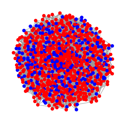
Let’s look at an example where we randomly assign nodes to group labels in a network#
Is our approach able to correctly estimate the proportion of red/blue nodes?
N = 1000
G = nx.barabasi_albert_graph(N,10)
pos = nx.spring_layout(G)
print("Average degree: %1.1f" % np.mean(list(dict(G.degree()).values())))
M = G.number_of_edges()
print("Number of edges:", M)
Average degree: 19.8
Number of edges: 9900
prob_red = 0.7
reds = 0
blues = 0
for node in G.nodes():
    G.nodes[node]['team'] = 'red' if np.random.rand() < prob_red else 'blue'
    if G.nodes[node]['team'] == 'red':
        reds += 1
    else:
        blues += 1

print("Number of red nodes:",reds)
print("Number of blue nodes:",blues)

fig, ax = plt.subplots(1,1,figsize=(5,5),dpi=100)
nx.draw(G, pos=pos, node_color=nx.get_node_attributes(G, 'team').values(),ax=ax,node_size=50, edge_color='.6')
plt.show()
Number of red nodes: 707
Number of blue nodes: 293
from scipy.special import binom

def prob_i(N_e, k_i, n):
    """
    Calculate the probability of at least one sample overlapping with node i.

    Parameters:
    N_e : int
        Effective size of the network.
    k_i : int
        Number of samples that do not include node i.
    n : int
        Number of nodes in the sample.

    Returns:
    float
        Probability of at least one sample overlapping with node i.
    """
    # If the sample size exceeds the available nodes excluding k_i,
    # the probability is 1 (certain inclusion).
    if n > N_e - k_i:
        return 1.0

    # Otherwise, calculate the complement of the probability that node i is not sampled.
    return 1.0 - binom(N_e - k_i, n) / binom(N_e, n)
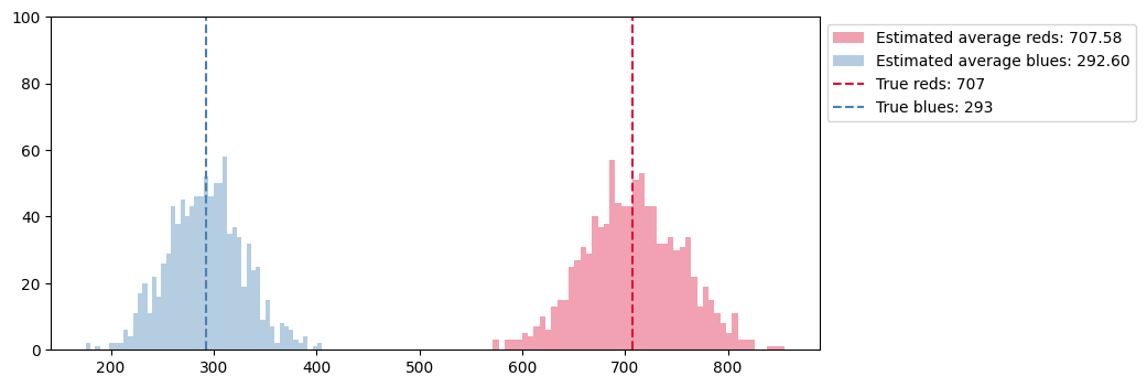
# We use the Horovitz-Thompson estimator to get those numbers from sampled graphs
B = 1000
reds_est = [None]*B
blues_est = [None]*B
degrees = dict(G.degree())

for b in range(B):
    n = 100
    G_s = incident_subgraph_sampling(G,n)
    V_s = list(G_s.nodes())
    E_s = list(G_s.edges())
    pi = {node: prob_i(M,degrees[node],n)  for node in V_s}
    reds_est[b] = sum([ 1.0/pi[node] for node in V_s if G.nodes[node]['team'] == 'red'])
    blues_est[b] = sum([ 1.0/pi[node] for node in V_s if G.nodes[node]['team'] == 'blue'])
fig, ax = plt.subplots(1,1,figsize=(9,4),dpi=100)

ax.hist(reds_est, bins=50, color='crimson', alpha=0.4,
        label='Estimated average reds: %.2f'%(np.mean(reds_est)))
ax.hist(blues_est, bins=50, color='steelblue', alpha=0.4,
        label='Estimated average blues: %.2f'%(np.mean(blues_est)))

ax.vlines(reds, 0, 100, color='crimson', ls='--', label='True reds: %i'%reds)
ax.vlines(blues, 0, 100, color='steelblue', ls='--', label='True blues: %i'%blues)

ax.legend(loc=2,bbox_to_anchor=[1.0,1.0])
ax.set_ylim(0,100)

plt.show()
N = 10000
M = 50000
G = nx.gnm_random_graph(N,M)
degrees = list(dict(G.degree()).values())
print("Average degree: %1.3f" % np.mean(degrees))
n = 5000
Average degree: 10.000
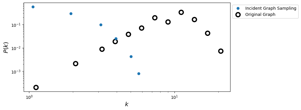
# Using Incident Graph Sampling
G_incid = incident_subgraph_sampling(G, n)
degrees_incid = list(dict(G_incid.degree()).values())
x_incid, y_incid = get_binning(degrees_incid, log_binning=True, is_pmf=True, num_bins=15)
# True Degree distribution
x_true, y_true = get_binning(degrees, log_binning=True, is_pmf=True, num_bins=15)
fig, ax = plt.subplots(1,1,figsize=(9,4),dpi=100)

ax.loglog(x_incid, y_incid, 'o', label='Incident Graph Sampling')
ax.scatter(x_true, y_true, s= 100, facecolors='none', edgecolors='k', lw=3, label = 'Original Graph')

ax.legend(loc=2,bbox_to_anchor=[1.0,1.0])
ax.set_xlabel(r'$k$',fontsize='x-large')
ax.set_ylabel(r'$P(k)$',fontsize='x-large')


plt.show()
Method 3: Edge Sampling with Graph Induction (ES-i)#
Edge Sampling with Graph Induction consists in drawing at random \(n\) edges from a graph of size \(N\). Let us denote with \(G = (V,E)\) the original graph and with \(G_s = (V_s,E_s)\) the sampled subgraph. Then, \(V_s\) contains all the nodes incident to the randomly selected edges and \(E_s\) comprises the \(n\) edges randomly selected from \(E\) plus all the other edges \(e_{i,j} \in E\) such that that both \(i\) and \(j\) belong to \(V_s\).
Source: Ahmed, N., Neville, J., & Kompella, R. R. (2011). Network sampling via edge-based node selection with graph induction. https://docs.lib.purdue.edu/cstech/1747/
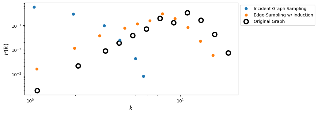
Some observations:
Edge sampling is inherently biased towards selection of nodes with higher degrees resulting in an upward bias in the degree distributions of sampled nodes compared to nodes in the original graph.
In sampled subgraphs degrees are naturally underestimated since only a fraction of neighbors may be selected. This results in a downward bias, regardless of the actual sampling algorithm used.
The upward bias of edge sampling can help offset this downward bias to some extent, it alone is not sufficient to fully offset the bias.
Then, a simple graph induction step over the edge-sampled node set (where we sample all the edges between any sampled nodes in the graph) can recover much of the connectivity around the high degree nodes offsetting the downward degree bias as well as improving local clustering in the sampled graph.
def edge_sampling_with_induction(G, n):
    """
    Perform edge sampling with induction and return a new graph.

    Parameters:
    G : networkx.Graph
        Input graph.
    n : int
        Number of edges to sample initially.

    Returns:
    networkx.Graph
        A new graph induced by the sampled nodes and edges.
    """
    # Get all edges and total number of edges in the graph
    edges = list(G.edges())
    M = G.number_of_edges()

    # Sample n edges randomly without replacement
    sampled_edges = set([edges[i] for i in np.random.permutation(M)[:n]])

    # Extract the set of nodes in the sampled edges
    nodes_from_sampled_edges = set(node for edge in sampled_edges for node in edge)

    # Induce edges between the sampled nodes
    induced_edges = set(sampled_edges)
    for node_i, node_j in edges:
        if node_i in nodes_from_sampled_edges and node_j in nodes_from_sampled_edges:
            induced_edges.add((node_i, node_j))

    # Create a new graph with the sampled nodes and induced edges
    new_graph = nx.Graph()
    new_graph.add_nodes_from(nodes_from_sampled_edges)
    new_graph.add_edges_from(induced_edges)

    return new_graph
G_esi = edge_sampling_with_induction(G, n)
degrees_esi = list(dict(G_esi.degree()).values())
x_esi,y_esi = get_binning(degrees_esi, log_binning=True, is_pmf=True, num_bins=15)
fig, ax = plt.subplots(1,1,figsize=(9,4),dpi=100)

ax.loglog(x_incid, y_incid, 'o', label='Incident Graph Sampling')
ax.loglog(x_esi, y_esi, 'o', label='Edge-Sampling w/ Induction')
ax.scatter(x_true, y_true, s= 100, facecolors='none', edgecolors='k', lw=3, label = 'Original Graph')

ax.legend(loc=2,bbox_to_anchor=[1.0,1.0])
ax.set_xlabel(r'$k$',fontsize='x-large')
ax.set_ylabel(r'$P(k)$',fontsize='x-large')


plt.show()
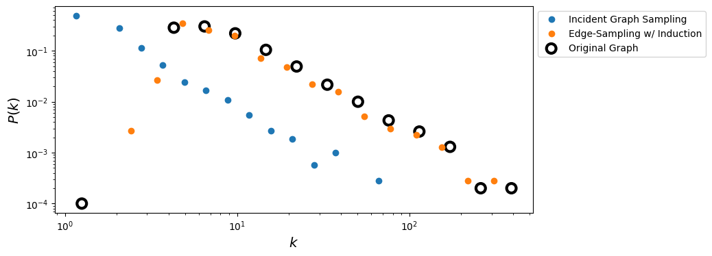
But what about in networks with heavy-tail degree distributions?#
N = 10000
ba = nx.barabasi_albert_graph(N, 5)
degrees = np.array(list(dict(ba.degree()).values()))
print("Average degree: %1.3f" % np.mean(degrees))
M = ba.number_of_edges()
n = int(M*0.15)
Average degree: 9.995
# Using Edge Sampling with Graph Induction
ba_s = edge_sampling_with_induction(ba,n)
V_s, E_s = ba_s.number_of_nodes(), ba_s.number_of_edges()
degrees_s = np.array(list(dict(ba_s.degree()).values()))

x_s,y_s = get_binning(degrees_s, log_binning=True, is_pmf=True, num_bins=15)
# Using Incident Graph Sampling
ba_s_i = incident_subgraph_sampling(ba,n)
V_s_i, E_s_i = ba_s_i.number_of_nodes(), ba_s_i.number_of_edges()
degrees_s_i = np.array(list(dict(ba_s_i.degree()).values()))

x_s_i,y_s_i = get_binning(degrees_s_i, log_binning=True, is_pmf=True, num_bins=15)
# True Degree distribution
x_t,y_t = get_binning(degrees, log_binning=True, is_pmf=True, num_bins=15)
fig, ax = plt.subplots(1,1,figsize=(9,4),dpi=100)

ax.loglog(x_s_i,y_s_i,'o', label = 'Incident Graph Sampling')
ax.loglog(x_s,y_s,'o', label='Edge-Sampling w/ Induction')
ax.scatter(x_t,y_t, s= 100, facecolors='none', edgecolors='k', lw=3, label = 'Original Graph')

ax.legend(loc=2,bbox_to_anchor=[1.0,1.0])
ax.set_xlabel(r'$k$',fontsize='x-large')
ax.set_ylabel(r'$P(k)$',fontsize='x-large')


plt.show()
from scipy.stats import ks_2samp

def ks_d(values1, values2):
    """
    Compute the Kolmogorov-Smirnov (KS) statistic to compare two distributions.

    Parameters:
    values1 : array-like
        First sample of values.
    values2 : array-like
        Second sample of values.

    Returns:
    float
        KS statistic (D), representing the maximum distance between the empirical
        cumulative distribution functions (ECDFs) of the two samples.
    """
    D, _ = ks_2samp(values1, values2)
    return D

print('Original vs Edge Sampling w/ Induction:\t', ks_d(degrees, degrees_s))
print('Original vs Incident Graph Sampling:\t', ks_d(degrees, degrees_s_i))
Original vs Edge Sampling w/ Induction:	 0.15294249611746435
Original vs Incident Graph Sampling:	 0.9359672077459775
Why is this working better?#
Standard edge sampling (i.e. incident subgraph sampling) is biased towards selection of high degree nodes. Therefore, the sampled degree distribution is upward biased with respect to the original graph. However, in all sampled subgraphs, degrees are actually underestimated because only a fraction of neighbors may be selected.
As a consequence, there is a downward bias, regardless of the actual sampling algorithm used. Incident subgraph sampling alone is not enough to correct for this downward bias since it samples each edge independently and it is therefore unlikely to preserve local nodes connectivity.
By adding the additional graph induction step, not only local clustering is improved, but it is also easier to reconstruct the connectivity of (high degree) nodes.
Method 4: Star Sampling#
Star sampling consists in drawing at random \(n\) nodes from a graph of order \(N\). Let us denote this initial set of nodes with \(V_{s0}\). Then, a set of edges \(E_s\) is created including all the edges which are incident to the vertices in \(V_{s0}\). Then, two different sampling designs can be employed:
Unlabeled star sampling: the sampled graph is simply \(G_s = (V_s,E_s)\) with \(V_{s}=V_{s0}\),
Labeled star sampling: the sampled graph includes all the nodes \(j\) incident to the edges in \(E_s\). That is, the original set \(V_{s0}\) is extended. Therefore, the sampled graph is \(G_s = (V_s,E_s)\).
In both cases the edge inclusion probabilities is equal to: \( \pi_{e_{i,j}} = 1 - \frac{\binom{N-2}{n}}{\binom{N}{n}}\) while the vertex inclusion probabilities differ (see Section 5.3.2 in “Statistical Analysis of Network Data: Methods and Models”, 2009).
def labeled_star_sampling(G, n):
    """
    Labeled star sampling on a NetworkX graph.

    Parameters
    ----------
    G : networkx.Graph or networkx.DiGraph
        Input graph of order N.
    n : int
        Number of nodes to select uniformly at random for V_{s0}.

    Returns
    -------
    G_s : networkx.Graph or networkx.DiGraph
        Sampled graph G_s = (V_s, E_s) where:
        - V_{s0} is a random subset of n nodes,
        - E_s contains all edges incident to nodes in V_{s0},
        - V_s includes V_{s0} plus all neighbors of V_{s0}
          (i.e., labeled star sampling).
    """
    # Handle empty graph
    if G.number_of_nodes() == 0:
        return nx.DiGraph() if G.is_directed() else nx.Graph()

    nodes = list(G.nodes())
    shuffle(nodes)

    # Ensure n doesn't exceed |V|
    n = min(n, len(nodes))

    # Initial random set V_{s0}
    V_s0 = set(nodes[:n])

    # Initialize sampled graph with same directedness as G
    G_s = nx.DiGraph() if G.is_directed() else nx.Graph()

    # Add all edges incident to V_{s0}; NetworkX will automatically
    # include the corresponding endpoint nodes, so this yields V_s.
    for u in V_s0:
        for v in G.neighbors(u):
            G_s.add_edge(u, v)

    # Make sure all sampled centers are present even if isolated
    G_s.add_nodes_from(V_s0)

    return G_s
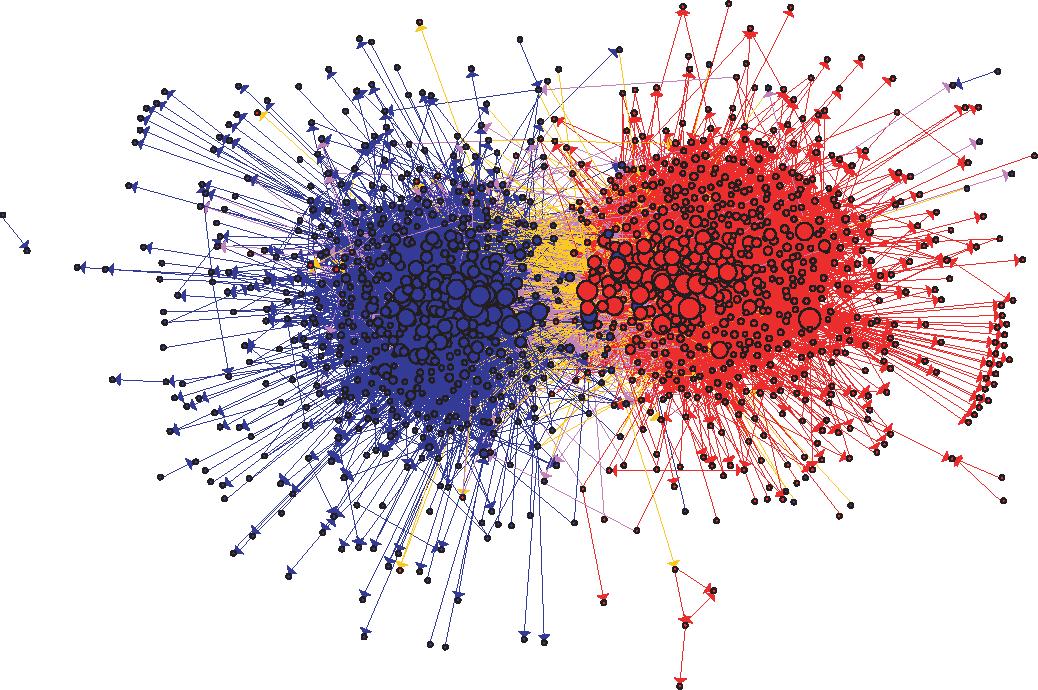
Let us use the Political Blogs dataset#
In this example, we are going to use the a directed graph which includes a collection of hyperlinks between weblogs on US politics, recorded in 2005 by Adamic and Glance (L. A. Adamic and N. Glance, “The political blogosphere and the 2004 US Election”, in Proceedings of the WWW-2005 Workshop on the Weblogging Ecosystem (2005)).
Recall that the data are included in two tab-separated files:
polblogs_nodes.tsv: node id, node label, political orientation (0 = left or liberal, 1 = right or conservative).
polblogs_edges.tsv: source node id, target node id.
nodes = dict()
with open('data/polblogs_nodes_class.tsv','r') as fp:
for line in fp:
node_id, node_label, pol_or = line.strip().split('\t')
nodes[int(node_id)] = {'label': node_label, 'political': int(pol_or)}
edges = []
with open('data/polblogs_edges_class.tsv','r') as fp:
for line in fp:
source_node_id, target_node_id = map(int,line.strip().split('\t'))
edges.append((source_node_id, target_node_id))
AG_net = nx.Graph()
AG_net.add_nodes_from(nodes)
AG_net.add_edges_from(edges)
print('Number of edges: %i' % AG_net.number_of_edges())
print('Number of nodes: %i' % AG_net.number_of_nodes())
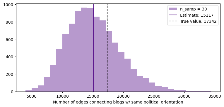
same_political_orientation = sum([ 1 for node_i,node_j in edges
if nodes[node_i]['political'] == nodes[node_j]['political'] ])
print("Number of edges connecting blogs with the same political orientation:", same_political_orientation)
Number of edges: 16718
Number of nodes: 1490
Number of edges connecting blogs with the same political orientation: 17342
# helper functions for the math

from scipy.special import binom, factorial, gamma

def approx_log_binom(n,m):
    # using the fact that ln(n!) ~ n ln(n) - n + O(ln(n))
    return n*np.log(n)-m*np.log(m)-(n-m)*np.log(n-m)

def prob_i(N_e,k_i,n):
    if n>N_e-k_i:
        pi_i = 1.0
    else:
        pi_i = 1 - binom(N_e-k_i,n) / binom(N_e,n)
    return pi_i

def approx_prob_i(N_e,k_i,n):
    if n > N_e-k_i:
        pi_i = 1.0
    else:
        pi_i = 1.0 - np.exp(approx_log_binom(N_e-k_i,n)-approx_log_binom(N_e,n))
    return pi_i
n_iter = 10000
same_political_orientation_est = np.zeros(n_iter)
N = AG_net.number_of_nodes()
M = AG_net.number_of_edges()
N_v = []
N_e = []
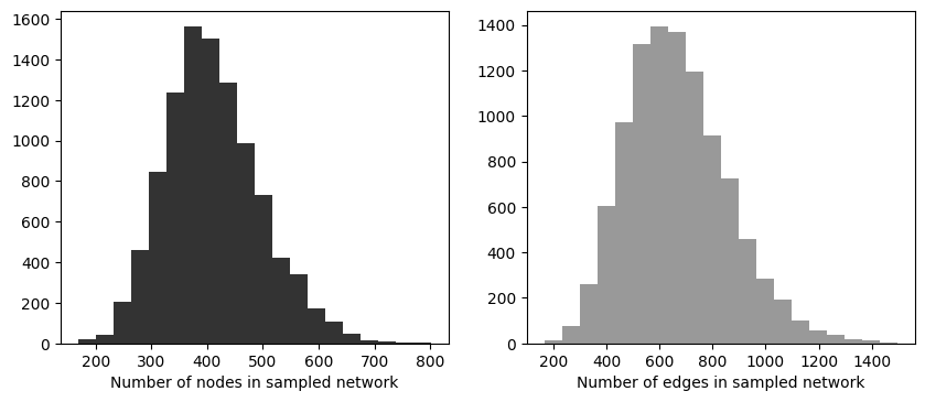
for b in range(n_iter):
n = 30
G_s = labeled_star_sampling(AG_net, n)
V_s = list(G_s.nodes())
E_s = list(G_s.edges())
prob_eij = 1.0 - np.exp(approx_log_binom(N-2, n) - approx_log_binom(N, n))
N_v.append(len(V_s))
N_e.append(len(E_s))
same_political_orientation_est[b] = sum([ 1.0/prob_eij for node_i,node_j in E_s
if nodes[node_i]['political'] == nodes[node_j]['political'] ])
fig, ax = plt.subplots(1,2,figsize=(10,4),dpi=100)
ax[0].hist(N_v,bins=20,color='.2')
ax[1].hist(N_e,bins=20,color='.6')

ax[0].set_xlabel('Number of nodes in sampled network')
ax[1].set_xlabel('Number of edges in sampled network')

plt.show()
fig, ax = plt.subplots(1,1,figsize=(9,4),dpi=100)

ax.hist(same_political_orientation_est,30,color='indigo', alpha=0.4, label='n_samp = %i'%n)

ylims = ax.get_ylim()
ax.vlines(np.mean(same_political_orientation_est), 0, ylims[1]*1.1, color='indigo', ls='-',
          label="Estimate: %.0f"%np.mean(same_political_orientation_est))
ax.vlines(same_political_orientation, 0, ylims[1]*1.1, color='k', ls='--',
          label="True value: %i"%same_political_orientation)

ax.set_xlabel('Number of edges connecting blogs w/ same political orientation')

ax.legend()
ax.set_ylim(0, ylims[1])


plt.show()
Method 5: Snowball Sampling#
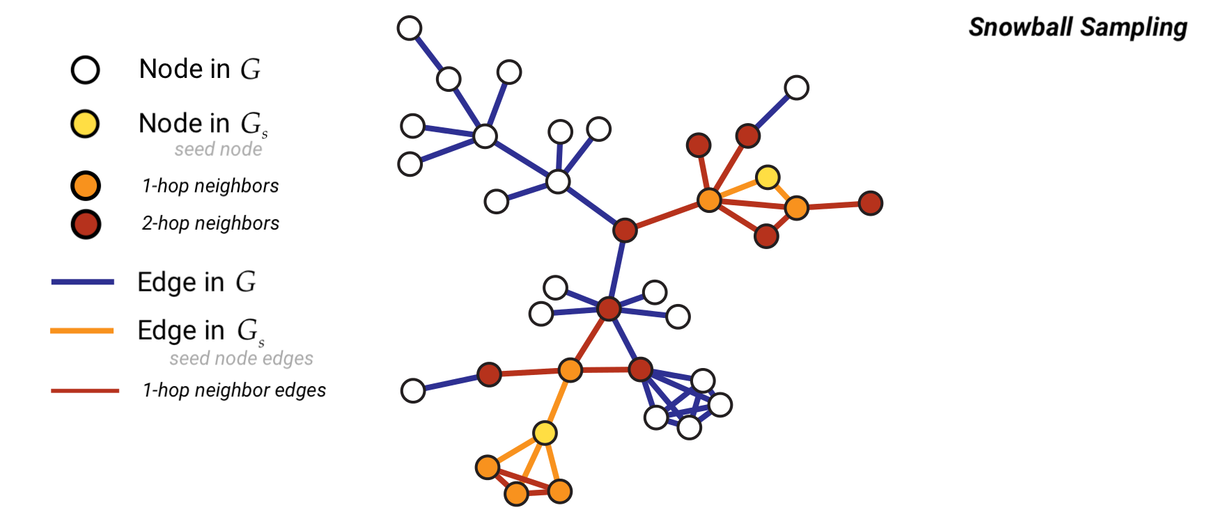
Snowball sampling consists of drawing at random \(n\) nodes from a graph of size \(N\). Let’s denote this initial set of nodes with \(V_{s,0}\) and with \(\mathbb{V}(S)\) the set of all neighbors of the vertices in the a given set \(S\). Then, a \(k\)-wave snowball sampling algorithm simply extends the initial set of nodes \(V_{s,0}\) \(k\) times in the following way:
\(V_{s,1} = \mathbb{V}(V_{s,0}) \cap \bar{V}_{s,0}\),
\(V_{s,2} = \mathbb{V}(V_{s,1}) \cap \bar{V}_{s,1} \cap \bar{V}_{s,0}\),
…
\(V_{s,k} = \mathbb{V}(V_{s,k-1}) \cap \bar{V}_{s,k-1} \cap \dots \cap \bar{V}_{s,0}\).
When the degree distribution of the original network is power-law, it is found that the estimated degree exponent decreases with snowball sampling as we decrease the sampling fraction.
Sampled networks are shown to be more disassortative than the original networks. This pattern is common no matter whether the original network is assortative, disassortative, or neutral.
def snowball_sampling(G, seed_nodes, n_waves=2):
    """
    Perform snowball sampling on a graph.

    Parameters:
    G : networkx.Graph or networkx.DiGraph
        Input graph.
    seed_nodes : list or set
        Initial set of nodes to start the snowball sampling.
    n_waves : int, optional
        Number of waves to expand the snowball sampling (default is 2).

    Returns:
    networkx.Graph or networkx.DiGraph
        A new graph G_s containing the sampled nodes and edges.
    """
    # Initialize sets to keep track of sampled nodes and edges
    V_s = set(seed_nodes)
    E_s = set()

    # Initialize the wave structure
    V = [set()] * (n_waves + 1)
    V[0] = set(seed_nodes)

    # Perform snowball sampling over the specified number of waves
    for k in range(n_waves):
        V[k + 1] = set()  # Initialize the next wave
        for node_i in V[k]:
            for node_j in G.neighbors(node_i):
                # Add the edge to the sampled edge set
                edge = (node_i, node_j) if not G.is_directed() and node_i < node_j else (node_i, node_j)
                E_s.add(edge)

                # Add the neighboring node to the next wave
                V[k + 1].add(node_j)

        # Exclude nodes already in the sampled set
        V[k + 1] -= V_s

        # Add new nodes to the sampled set
        V_s.update(V[k + 1])

    # Create the new sampled graph
    G_s = G.subgraph(V_s).copy()

    return G_s
N = 15000
m = 3
G = nx.barabasi_albert_graph(N, m)
M = G.number_of_nodes()
degrees = list(dict(G.degree()).values())
print(M)
15000
fig, ax = plt.subplots(1,1,figsize=(9, 4), dpi=100)

n = 50  # Number of seed nodes
n_waves = 5  # Maximum number of waves
degrees_sampled = [None] * (n_waves + 1)

nodes = list(G.nodes())

# Perform snowball sampling for increasing numbers of waves
for k in range(n_waves + 1):
    # Select seed nodes randomly
    seed_nodes = set(np.random.choice(nodes, size=n, replace=False))

    # Perform snowball sampling
    G_s = snowball_sampling(G, seed_nodes, n_waves=k)

    # Print summary of the sampled graph
    print(f"Number of waves: {k} | Number of nodes discovered: {G_s.number_of_nodes()} | "
          f"Number of edges discovered: {G_s.number_of_edges()}")

    # Get degree distribution of the sampled graph
    degrees_sampled[k] = [deg for _, deg in G_s.degree()]

    # Plot degree distribution for the current wave
    if k > 0:
        x1, y1 = get_binning(degrees_sampled[k], log_binning=True, num_bins=15, is_pmf=False)
        ax.loglog(x1, y1, '--o', label=f'Wave: {k}')

# Plot the degree distribution of the original graph
x, y = get_binning(degrees, log_binning=True, num_bins=15, is_pmf=False)
ax.scatter(x, y, s=100, facecolors='none', edgecolors='k', lw=3, label='Original Graph')

ax.legend(loc=2,bbox_to_anchor=[1.0,1.0])
ax.set_xlabel(r'$k$',fontsize='x-large')
ax.set_ylabel(r'$P(k)$',fontsize='x-large')


plt.show()
Number of waves: 0 | Number of nodes discovered: 50 | Number of edges discovered: 1
Number of waves: 1 | Number of nodes discovered: 376 | Number of edges discovered: 436
Number of waves: 2 | Number of nodes discovered: 4630 | Number of edges discovered: 10444
Number of waves: 3 | Number of nodes discovered: 13310 | Number of edges discovered: 39162
Number of waves: 4 | Number of nodes discovered: 15000 | Number of edges discovered: 44991
Number of waves: 5 | Number of nodes discovered: 15000 | Number of edges discovered: 44991
Method 6: Traceroute Sampling#
Traceroute sampling is an example of a link tracing algorithm used to generate sampled graphs. In traceroute sampling, two initial disjoint sets of nodes are drawn at random: a set of sources \(V_S\) of size \(n_S\) and a set of targets \(V_T\) of size \(n_T\). Then, a route is traced from each node in \(V_S\) to each node in \(V_T\) and all vertices and edges encountered are added to \(V_s\) and \(E_s\), respectively. Then, the sampled graph is \(G_s = (V_s,E_s)\).
If the source and target sets are obtained using a simple random sampling without replacement and the route considered is simply the shortest path between each pair of vertices, then the vertex inclusion probability can be approximated with:
while the edge inclusion probability can be approximated with:
where \(b_i\) is the betweenness centrality of vertex \(i\) and \(b_{e_{i,j}}\) is the betweenness centrality of edge \(e_{i,j}\).
Traceroute sampling can make power laws appear where none existed in the underlying graph (even in the extreme case of regular random graphs)
Even when the original degree distribution is power-law, traceroute sampling significantly underestimate the tail exponent
def traceroute_sampling(G, n_sources=5, n_targets=50):
    """
    Perform traceroute sampling on a graph, selecting multiple sources and targets.

    Parameters:
    G : networkx.Graph
        Input graph.
    n_sources : int, optional
        Number of source nodes (default is 5).
    n_targets : int, optional
        Number of target nodes (default is 50).

    Returns:
    networkx.Graph
        A new graph containing the sampled nodes and edges.
    """
    nodes = list(G.nodes())
    shuffle(nodes)

    # Select sources and targets
    sources = set(nodes[:n_sources])
    targets = set(nodes[n_sources:n_sources + n_targets])

    # Initialize the sampled graph
    G_s = nx.Graph() if not G.is_directed() else nx.DiGraph()

    # Compute shortest paths from each source to each target
    for source_node in sources:
        for target_node in targets:
            try:
                path = nx.shortest_path(G, source=source_node, target=target_node)
                G_s.add_nodes_from(path)
                G_s.add_edges_from((path[i], path[i + 1]) for i in range(len(path) - 1))
            except nx.NetworkXNoPath:
                pass  # Ignore if no path exists

    return G_s
N = 2000
k = 15.0
G = nx.erdos_renyi_graph(N, k/(N-1))
degrees = list(dict(G.degree()).values())
M = G.number_of_edges()

G_s_t = traceroute_sampling(G, n_sources=2, n_targets=3)
n_sources = 8
share_nodes = []
share_edges = []
sampled_degrees = []

N_targets = np.arange(50,261,50)
for n_targets in N_targets:
    G_s = traceroute_sampling(G, n_sources, n_targets)
    share_nodes.append(G_s.number_of_nodes()/N)
    share_edges.append(G_s.number_of_edges()/M)

    degrees_s = list(dict(G_s.degree()).values())

    sampled_degrees.append(degrees_s)

fig, ax = plt.subplots(1,1,figsize=(9, 4), dpi=100)
for k, values in enumerate(sampled_degrees):
    x,y = get_binning(values, log_binning=True, num_bins=15, is_pmf=True)
    ax.loglog(x,y, 'o--', label = "Number of targets: %d" % N_targets[k])

x,y = get_binning(degrees, log_binning=True, num_bins=15, is_pmf=False)
ax.scatter(x,y, s= 100, facecolors='none', edgecolors='k',lw=3,label = "Original Graph")

ax.legend(loc=2,bbox_to_anchor=[1.0,1.0])
ax.set_xlabel(r'$k$',fontsize='x-large')
ax.set_ylabel(r'$P(k)$',fontsize='x-large')


plt.show()
Bias reduction in Traceroute Sampling#
We can use the capture-recapture estimator to improve the sampled degree distribution (from Flaxman & Vera, 2007).
Let us denote with \(U\) the set of sources we are using to perform the traceroute sampling and with \(G_{u_1}\) and \(G_{u_2}\) two sampled graphs obtained using source nodes \(u_1\) and \(u_2\), respectively. Then, we can estimate the degree of a generic node \(i\) in the sampled graph \(G_{u_1}\) as:
Then, we can repeat the same procedure for all the pairs of sources in \(U\) and obtain the final estimate for the degree of node \(i\) as:
Source: Flaxman, A. D., & Vera, J. (2007). Bias reduction in traceroute sampling–towards a more accurate map of the internet. In International Workshop on Algorithms and Models for the Web-Graph (pp. 1-15). Berlin, Heidelberg: Springer Berlin Heidelberg. https://link.springer.com/chapter/10.1007/978-3-540-77004-6_1
from collections import defaultdict
from itertools import combinations

def bias_reduction(sampling_method, num_samples, args):
    """
    sampling_method(**args) should return a NetworkX graph G_s
    for each sample (e.g., traceroute sample from some source set).
    """
    # Draw samples (each is a NetworkX graph)
    samples = [sampling_method(**args) for _ in range(num_samples)]
    degrees = defaultdict(list)

    # Pair up samples: first half vs second half
    # (num_samples should be even for this scheme)
    pairs = list(zip(samples[:num_samples // 2], samples[num_samples // 2:]))

    # If you prefer all pairs, use: pairs = combinations(samples, 2)
    for G_s1, G_s2 in pairs:
        # For each node in first sampled graph
        for u in G_s1.nodes():
            if u in G_s2:
                # Neighbors in each sampled graph
                neigh1 = set(G_s1.neighbors(u))
                neigh2 = set(G_s2.neighbors(u))

                N_c = len(neigh1.intersection(neigh2))
                if N_c > 2:
                    # capture–recapture estimator for k(u)
                    degrees[u].append(len(neigh1) * len(neigh2) / N_c)

    # Median estimate per node
    degrees_est = [np.median(values) for node, values in degrees.items()]

    return degrees_est
n_sources = 10
n_targets = 150
n_samples = 10

args = {'G':G,'n_sources':n_sources,'n_targets':n_targets}

G_s = traceroute_sampling(G,n_sources,n_targets)
degrees_s = list(dict(G_s.degree()).values())


fig, ax = plt.subplots(1,1,figsize=(9, 4), dpi=100)

# k = N_targets[2]
# values = sampled_degrees[2]
for k, values in enumerate(sampled_degrees):
    x,y = get_binning(values, log_binning=True, num_bins=12, is_pmf = True)
    ax.loglog(x,y, 'o--', label = "Number of targets: %d" % N_targets[k])

degrees_est = bias_reduction(traceroute_sampling, n_samples, args)

x,y = get_binning(degrees_est, log_binning=True, num_bins=12, is_pmf = True)
ax.loglog(x,y, '-o', label = "Bias Correction")

x,y = get_binning(degrees, log_binning=True, num_bins=12, is_pmf = True)
ax.scatter(x,y, s= 100, facecolors='none', edgecolors='k',lw=3,label = "Original Graph")


ax.legend(loc=2,bbox_to_anchor=[1.0,1.0])
ax.set_xlabel(r'$k$',fontsize='x-large')
ax.set_ylabel(r'$P(k)$',fontsize='x-large')


plt.show()
There are many more ways to imagine debiasing the sampling procedure!
Method 7: Random Walk Sampling#
Random Walk sampling is another example of a link tracing algorithm used to generate sampled graphs. The classic algorithm works as follows:
We start from a random vertex \(i_0\);
At each \(t_{th}\) step of the walk, given that we are at node \(i_t\), we move to one of \(i_t\) neighbors with equal probability (i.e. if \(k_{i_t}\) is the degree of node \(i_t\), we pick one of its neighbors wiht probability \(1/k_{i_t}\)).
Then, \(V_s\) will include all the nodes visited during the random walk, while \(E_s\) will include all the edges traversed.
It can be shown that the probability of being at a particular node \(i\) converges to the stationary distribution:
In practice, we may allow for the fact that the graph is not connected and that our random walker might get stucked. If that is the case, we can randomly select a different starting node for the remaining steps. Lastly, we can allow for the possibility that the random walker “flies back” to the original node and re-starts walking from there.
def random_walk_sampling(G, n, fly_back=0.0, jump_after=10, v0=None):
    """
    Single-walker random walk sampling on a NetworkX graph,
    matching the logic of the adj_list-based random_walk_sampling.
    """
    if G.number_of_nodes() == 0:
        return nx.Graph() if not G.is_directed() else nx.DiGraph()

    nodes = list(G.nodes())

    if v0 is None:
        v0 = np.random.choice(nodes)

    V_s = {v0}
    E_s = set()
    stuck = 0

    node_t = v0
    nodes_discovered = len(V_s)
    edges_discovered = len(E_s)

    while len(V_s) < n:
        if np.random.rand() < fly_back:
            # Fly back to starting node
            next_node = v0
        else:
            neighbors = list(G.neighbors(node_t))
            if neighbors:
                next_node = np.random.choice(neighbors)
                # add node / edge as in adj_list version
                V_s.add(next_node)
                edge = (node_t, next_node) if node_t < next_node else (next_node, node_t)
                E_s.add(edge)
                node_t = next_node
            else:
                # no neighbors: we rely on stuck logic and teleports
                next_node = node_t  # no move

        # stuck logic: did we discover anything new?
        if (nodes_discovered == len(V_s)) and (edges_discovered == len(E_s)):
            stuck += 1
        else:
            stuck = 0

        nodes_discovered = len(V_s)
        edges_discovered = len(E_s)

        if stuck > jump_after:
            node_t = np.random.choice(nodes)
            V_s.add(node_t)
            stuck = 0

    # Build sampled graph
    G_s = nx.Graph() if not G.is_directed() else nx.DiGraph()
    G_s.add_nodes_from(V_s)
    G_s.add_edges_from(E_s)

    return G_s
N = 10000
m = 3
seed = 4
G = nx.barabasi_albert_graph(N, m, seed=seed)

# original degrees in the full graph
degrees_full_dict = dict(G.degree())
degrees_full = list(degrees_full_dict.values())
n = 3000
fly_back = 0.0

fig, ax = plt.subplots(1,1,figsize=(9, 4), dpi=100)

# sample with RW
G_s = random_walk_sampling(G, n, fly_back=fly_back)
V_s = list(G_s.nodes())

# degrees of sampled nodes in the *original* graph
deg_sampled_original = [degrees_full_dict[u] for u in V_s]

# binned curves
x, y = get_binning(deg_sampled_original,
                   log_binning=True, num_bins=15, is_pmf=False)
ax.loglog(x, y, marker='o', label='Fly_back: %f' % fly_back)

x0, y0 = get_binning(degrees_full, num_bins=15,
                     log_binning=True, is_pmf=False)
ax.scatter(x0, y0, s=100, facecolors='none', edgecolors='k', lw=3,
            label='Original')

ax.legend(loc=2,bbox_to_anchor=[1.0,1.0])
ax.set_xlabel(r'$k$',fontsize='x-large')
ax.set_ylabel(r'$P(k)$',fontsize='x-large')


plt.show()
Re-Weighted Random Walk#
One way to correct the bias towards high node degrees of the classic random walk is to re-weight the observed degree distribution of the sampled graph after running the random walk sampling:
Metropolis-Hastings Random Walk Sampling#
The classic random walk sampling algorithm is biased towards high degree nodes. One way to correct for this bias it to use Metropolis-Hastings random walk sampling.
Metropolis-Hastings random walk sampling algorithm works as follows:
we start from a random vertex \(i_0\);
at each \(t_{th}\) step of the walk, given that we are at node \(i_t\), we select at random one of \(i_t\) neighbors (let us denote this node with \(w\));
we generate a random number \(0\leq r \leq 1\);
if \(r \leq \frac{k_{i_t}}{k_{w}}\) then we accept the move, otherwise we stay at node \(i_t\) and we go back to 2.
Notice that - with this algorithm - the probability of sampling a node converges to the uniform distribution.
def metropolis_hastings_random_walk_sampling(G, n, fly_back=0.0, jump_after=10, v0=None):
    """
    Single-walker Metropolis–Hastings random walk sampling on a NetworkX graph.

    Mirrors the adj_list-based metropolis_hastings_random_walk_sampling:
    - start from v0 (or a random node),
    - propose a random neighbor,
    - accept with probability deg(curr) / deg(next),
    - use 'fly_back' and 'jump_after' as in the original code.
    """
    if G.number_of_nodes() == 0:
        return nx.Graph() if not G.is_directed() else nx.DiGraph()

    nodes = list(G.nodes())

    if v0 is None:
        v0 = np.random.choice(nodes)

    V_s = {v0}
    E_s = set()
    stuck = 0

    node_t = v0
    nodes_discovered = len(V_s)
    edges_discovered = len(E_s)

    while len(V_s) < n:
        if np.random.rand() < fly_back:
            # fly back to the starting node (no edge added)
            node_t = v0
        else:
            neighbors = list(G.neighbors(node_t))
            if neighbors:
                candidate = np.random.choice(neighbors)
                deg_curr = G.degree(node_t)
                deg_next = G.degree(candidate)

                if deg_next > 0:
                    if np.random.rand() < deg_curr / float(deg_next):
                        # accept move
                        V_s.add(candidate)
                        edge = (node_t, candidate) if node_t < candidate else (candidate, node_t)
                        E_s.add(edge)
                        node_t = candidate

            # stuck logic: did we discover anything new this iteration?
            if (nodes_discovered == len(V_s)) and (edges_discovered == len(E_s)):
                stuck += 1
            else:
                stuck = 0

            nodes_discovered = len(V_s)
            edges_discovered = len(E_s)

        if stuck > jump_after:
            # teleport to a random node
            node_t = np.random.choice(nodes)
            V_s.add(node_t)
            stuck = 0

    G_s = nx.Graph() if not G.is_directed() else nx.DiGraph()
    G_s.add_nodes_from(V_s)
    G_s.add_edges_from(E_s)

    return G_s
N = 15000
m = 3
seed = 4
G = nx.barabasi_albert_graph(N, m, seed=seed)

degrees_full_dict = dict(G.degree())
degrees_full = list(degrees_full_dict.values())

n = 2000
Fly_back = np.linspace(0.0, 0.3, 1)

fig, ax = plt.subplots(1,1,figsize=(9,4),dpi=100)

# Original degree distribution
x, y = get_binning(degrees_full, log_binning=True, num_bins=15, is_pmf=False)
ax.scatter(x, y, s=100, facecolors='none', ec='k', lw=3,
            label='Original Graph')

for k_idx, fly_back in enumerate(Fly_back):

    G_mh = metropolis_hastings_random_walk_sampling(G, n, fly_back=fly_back)
    V_mh = list(G_mh.nodes())

    degs_mh_sub = [d for _, d in G_mh.degree()]
    xs, ys = get_binning(degs_mh_sub, log_binning=True, num_bins=15, is_pmf=False)
    ax.loglog(xs, ys, '-o', label='Metropolis - Fly_back: %f' % fly_back)

    degs_mh_orig = [degrees_full_dict[u] for u in V_mh]
    xs_o, ys_o = get_binning(degs_mh_orig, log_binning=True, num_bins=15, is_pmf=False)
    ax.loglog(xs_o, ys_o, '-o', markersize=10,
               label='Original w Metropolis - Fly_back: %f' % fly_back)

    # random walk
    G_rw = random_walk_sampling(G, n, fly_back=fly_back)
    V_rw = list(G_rw.nodes())
    degs_rw_sub = [d for _, d in G_rw.degree()]
    xs_rw, ys_rw = get_binning(degs_rw_sub, log_binning=True, num_bins=15, is_pmf=False)
    ax.loglog(xs_rw, ys_rw, '-o', label='Random Walk - Fly_back: %f' % fly_back)

    degs_rw_orig = [degrees_full_dict[u] for u in V_rw]
    xs_rw_o, ys_rw_o = get_binning(degs_rw_orig, log_binning=True, num_bins=15, is_pmf=False)
    ax.loglog(xs_rw_o, ys_rw_o, '-o',
               label='Original w Random Walk - Fly_back: %f' % fly_back)


ax.legend(loc=2,bbox_to_anchor=[1.0,1.0])
ax.set_xlabel(r'$k$',fontsize='x-large')
ax.set_ylabel(r'$P(k)$',fontsize='x-large')


plt.show()
Next time…#
Link Prediction class_23_linkprediction.ipynb
References and further resources:#
Class Webpages
Jupyter Book: https://network-science-data-and-models.github.io/phys7332_fa25/README.html
Github: https://github.com/network-science-data-and-models/phys7332_fa25/
Syllabus and course details: https://brennanklein.com/phys7332-fall25
Achlioptas, D., Clauset, A., Kempe, D., & Moore, C. (2009). On the bias of traceroute sampling: Or, power-law degree distributions in regular graphs. Journal of the ACM (JACM), 56(4), 21.f Traceroute Sampling. In STOC, ACM (Vol. 1581139608, No. 05, p. 0005).
Ahmed, N. K., Neville, J., & Kompella, R. (2014). Network sampling: From static to streaming graphs. ACM Transactions on Knowledge Discovery from Data (TKDD), 8(2), 7.
Dall’Asta, L., Alvarez-Hamelin, I., Barrat, A., Vazquez, A., & Vespignani, A. (2004). A statistical approach to the traceroute-like exploration of networks: theory and simulations. arXiv preprint cond-mat/0406404.
Flaxman, A. D., & Vera, J. (2007). Bias Reduction in Traceroute Sampling–Towards a More Accurate Map of the Internet. In Algorithms and Models for the Web-Graph (pp. 1-15). Springer Berlin Heidelberg.
Gjoka, M., Kurant, M., Butts, C. T., & Markopoulou, A. (2010, March). Walking in Facebook: A case study of unbiased sampling of OSNs. In INFOCOM, 2010 Proceedings IEEE (pp. 1-9). IEEE.
Leskovec, J., & Faloutsos, C. (2006, August). Sampling from large graphs. In Proceedings of the 12th ACM SIGKDD international conference on Knowledge discovery and data mining (pp. 631-636). ACM.
Leskovec, J., Kleinberg, J., & Faloutsos, C. (2005, August). Graphs over time: densification laws, shrinking diameters and possible explanations. In Proceedings of the eleventh ACM SIGKDD international conference on Knowledge discovery in data mining (pp. 177-187). ACM.
Lovász, L. (1996). Random walks on graphs: A survey. Combinatorics, Paul Erdos is Eighty, 2, 353-398.
Kolaczyk, E. (2009). Statistical Analysis of Network Data: Methods and Models. Springer Series in Statistics.